Using eat for thermosensitivity analysis: Synthetic data#
The first examples uses synthetic (i.e. fake) to illustrate a typical thermo-sensitivity analysis.
[1]:
import matplotlib.pyplot as plt
from energy_analysis_toolbox.synthetic import DateSynthTSConsumption
[2]:
my_synthtisor = DateSynthTSConsumption(
    base_energy=1e3,
    ts_cool=5e1,
    ts_heat=1e2,
    noise_std=1e2,
    t_ref_cool=24,
    t_ref_heat=16,
)

data = my_synthtisor.random_consumption(start="2021-09-01", end="2024-04-17", size=None)
[3]:
fig, [ax1, ax2] = plt.subplots(1, 2, figsize=(10, 5))
data[["energy"]].plot(ax=ax1)
data[["T"]].plot(ax=ax1, secondary_y=True)
ax1.set_ylabel("Energy consumption (kWh)")
ax1.right_ax.set_ylabel("mean Daily Temperature (°C)")

data.plot.scatter(x="T", y="energy", ax=ax2)
ax2.set_xlabel("mean Daily Temperature (°C)")
ax2.set_ylabel("Energy consumption (kWh)")
ax1.set_title("Energy consumption and temperature over time")
ax2.set_title("Energy consumption vs temperature")
fig.suptitle("Synthetic data for energy consumption")
fig.tight_layout()
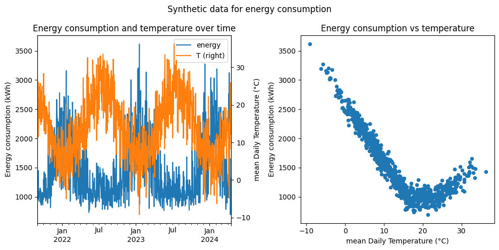
Thermo-sensitivity analysis#
The main objective of the analysis is to explain the impact of the temperature over the energy. In the case of the synthetic model, it relates to - finding the threshold temperatures for heating and cooling - finding the three coefficients \(E_0\), \(TS_{cooling}\) and \(TS_{heating}\) such that
[4]:
import pandas as pd
from energy_analysis_toolbox.weather.degree_days import dd_compute
[5]:
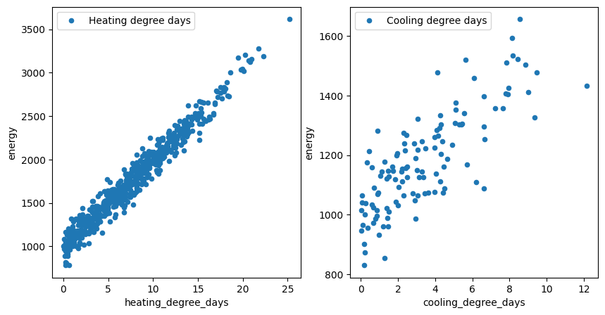
dd_heating = dd_compute(data["T"], reference=16, type="heating", method="mean")
dd_cooling = dd_compute(data["T"], reference=24, type="cooling", method="mean")
data_with_dd = pd.concat([data, dd_heating, dd_cooling], axis=1)
data_with_dd
[5]:
| base | thermosensitive | residual | energy | heating | ... | T | DD_heating | DD_cooling | heating_degree_days | cooling_degree_days | |
|---|---|---|---|---|---|---|---|---|---|---|---|
| 2021-09-01 | 1000.0 | 0.000000 | 161.687440 | 1161.687440 | 0.000000 | ... | 23.224711 | 0.000000 | 0.000000 | 0.000000 | 0.000000 |
| 2021-09-02 | 1000.0 | 0.000000 | 13.102712 | 1013.102712 | 0.000000 | ... | 16.387722 | 0.000000 | 0.000000 | 0.000000 | 0.000000 |
| 2021-09-03 | 1000.0 | 61.223187 | -100.234398 | 960.988789 | 0.000000 | ... | 25.224464 | 0.000000 | 1.224464 | 0.000000 | 1.224464 |
| 2021-09-04 | 1000.0 | 102.883927 | -10.972745 | 1091.911181 | 0.000000 | ... | 26.057679 | 0.000000 | 2.057679 | 0.000000 | 2.057679 |
| 2021-09-05 | 1000.0 | 451.955698 | -3.561074 | 1448.394624 | 451.955698 | ... | 11.480443 | 4.519557 | 0.000000 | 4.519557 | 0.000000 |
| ... | ... | ... | ... | ... | ... | ... | ... | ... | ... | ... | ... |
| 2024-04-13 | 1000.0 | 0.000000 | -304.763257 | 695.236743 | 0.000000 | ... | 21.235867 | 0.000000 | 0.000000 | 0.000000 | 0.000000 |
| 2024-04-14 | 1000.0 | 387.612615 | -61.604903 | 1326.007713 | 387.612615 | ... | 12.123874 | 3.876126 | 0.000000 | 3.876126 | 0.000000 |
| 2024-04-15 | 1000.0 | 95.981166 | 102.534803 | 1198.515969 | 0.000000 | ... | 25.919623 | 0.000000 | 1.919623 | 0.000000 | 1.919623 |
| 2024-04-16 | 1000.0 | 114.349285 | -31.728673 | 1082.620613 | 114.349285 | ... | 14.856507 | 1.143493 | 0.000000 | 1.143493 | 0.000000 |
| 2024-04-17 | 1000.0 | 0.000000 | -146.618598 | 853.381402 | 0.000000 | ... | 17.067412 | 0.000000 | 0.000000 | 0.000000 | 0.000000 |
960 rows × 11 columns
[6]:
fig, [ax1, ax2] = plt.subplots(1, 2, figsize=(10, 5))
data_with_dd[data_with_dd["heating_degree_days"] > 0].plot.scatter(
    x="heating_degree_days", y="energy", label="Heating degree days", ax=ax1
)
data_with_dd[data_with_dd["cooling_degree_days"] > 0].plot.scatter(
    x="cooling_degree_days", y="energy", ax=ax2, label="Cooling degree days"
);
Automatic calibration of the degree days model#
The degree days are computed relative to a reference (aka base) temperature.
This reference temperature corresponds to the temperature below (resp. above) which the heating (resp. cooling) is required. Hence, it depends on the building and the heating/cooling system.
Accordingly, the reference temperature is a parameter to be calibrated from the energy signature of the building.
[7]:
from energy_analysis_toolbox.thermosensitivity import ThermoSensitivity
[8]:
data.head()
[8]:
| base | thermosensitive | residual | energy | heating | cooling | T | DD_heating | DD_cooling | |
|---|---|---|---|---|---|---|---|---|---|
| 2021-09-01 | 1000.0 | 0.000000 | 161.687440 | 1161.687440 | 0.000000 | 0.000000 | 23.224711 | 0.000000 | 0.000000 |
| 2021-09-02 | 1000.0 | 0.000000 | 13.102712 | 1013.102712 | 0.000000 | 0.000000 | 16.387722 | 0.000000 | 0.000000 |
| 2021-09-03 | 1000.0 | 61.223187 | -100.234398 | 960.988789 | 0.000000 | 61.223187 | 25.224464 | 0.000000 | 1.224464 |
| 2021-09-04 | 1000.0 | 102.883927 | -10.972745 | 1091.911181 | 0.000000 | 102.883927 | 26.057679 | 0.000000 | 2.057679 |
| 2021-09-05 | 1000.0 | 451.955698 | -3.561074 | 1448.394624 | 451.955698 | 0.000000 | 11.480443 | 4.519557 | 0.000000 |
[9]:
my_synthtisor = DateSynthTSConsumption(
    base_energy=1e3,
    ts_cool=5e1,
    ts_heat=1e2,
    noise_std=1e2,
    t_ref_cool=24,
    t_ref_heat=16,
)

data = my_synthtisor.random_consumption(start="2021-09-01", end="2024-04-17", size=None)

ts = ThermoSensitivity(
    energy_data=data["energy"],
    temperature_data=data["T"],
    frequency="1D",
    degree_days_type="both",
    degree_days_computation_method="mean",  # here the provided data is already in daily frequency. Hence the only mean
)
[10]:
ts.calibrate_base_temperatures(xatol=1e-1, disp=True)
t0=13.8197, 15767.87, 295799.26
t0=16.1803, 10470.61, 295799.26
t0=17.6393, 12380.12, 295799.26
t0=16.2137, 10487.09, 295799.26
t0=15.7646, 10471.92, 295799.26
t0=16.0215, 10424.92, 295799.26
t0=15.9739, 10422.78, 295799.26
t0=15.9405, 10423.98, 295799.26

Optimization terminated successfully;
The returned value satisfies the termination criteria
(using xtol =  0.1 )
t0=23.8197, 9776.37, 28378.26
t0=26.1803, 12393.81, 28378.26
t0=22.3607, 9939.09, 28378.26
t0=23.2647, 9690.19, 28378.26
t0=23.2981, 9689.96, 28378.26
t0=23.3314, 9690.53, 28378.26

Optimization terminated successfully;
The returned value satisfies the termination criteria
(using xtol =  0.1 )
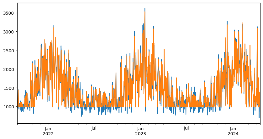
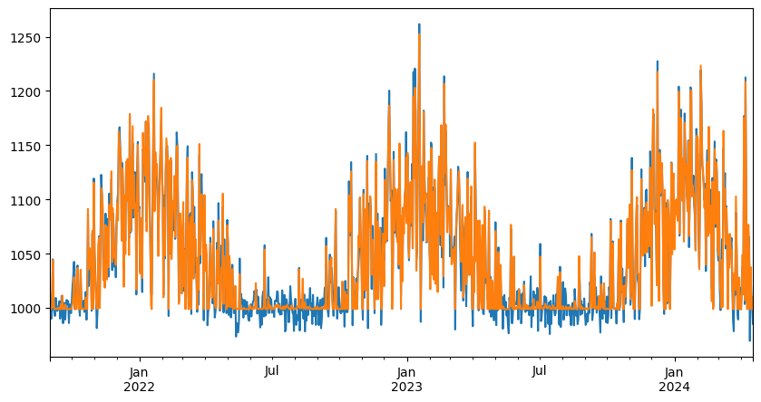
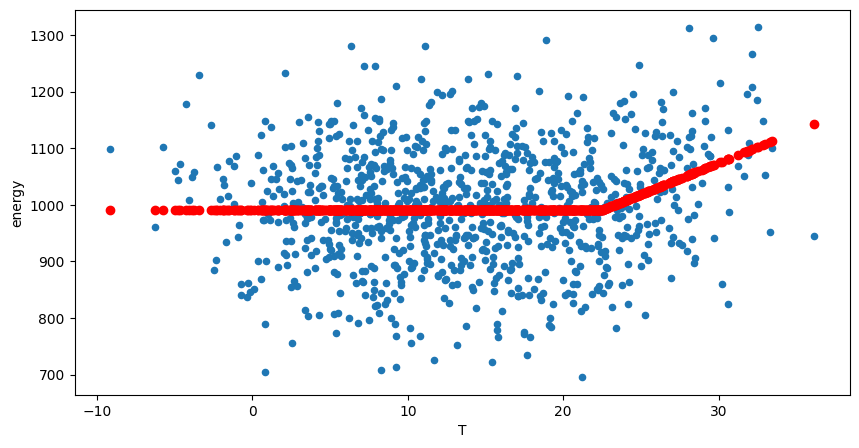
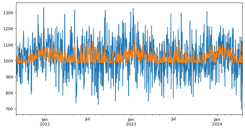
Fitting thermo-sensitivity model#
using the newlly computed degree days, we can fit the thermo-sensitivity model to the energy consumption.
[11]:
ts.fit()
ts.model.summary()
[11]:
| Dep. Variable: | energy | R-squared: | 0.964 |
|---|---|---|---|
| Model: | OLS | Adj. R-squared: | 0.964 |
| Method: | Least Squares | F-statistic: | 1.266e+04 |
| Date: | Fri, 11 Oct 2024 | Prob (F-statistic): | 0.00 |
| Time: | 20:46:09 | Log-Likelihood: | -5793.0 |
| No. Observations: | 960 | AIC: | 1.159e+04 |
| Df Residuals: | 957 | BIC: | 1.161e+04 |
| Df Model: | 2 | ||
| Covariance Type: | nonrobust |
| coef | std err | t | P>|t| | [0.025 | 0.975] | |
|---|---|---|---|---|---|---|
| heating_degree_days | 101.0069 | 0.640 | 157.815 | 0.000 | 99.751 | 102.263 |
| cooling_degree_days | 48.4614 | 2.057 | 23.554 | 0.000 | 44.424 | 52.499 |
| Intercept | 986.7006 | 4.709 | 209.553 | 0.000 | 977.460 | 995.941 |
| Omnibus: | 1.113 | Durbin-Watson: | 1.993 |
|---|---|---|---|
| Prob(Omnibus): | 0.573 | Jarque-Bera (JB): | 1.180 |
| Skew: | -0.077 | Prob(JB): | 0.554 |
| Kurtosis: | 2.926 | Cond. No. | 10.4 |
Notes:
[1] Standard Errors assume that the covariance matrix of the errors is correctly specified.
[12]:
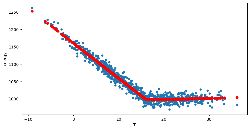
pred = ts.model.predict()

fig, ax = plt.subplots(figsize=(10, 5))
data["energy"].plot(ax=ax, label="Observed")
ax.plot(data.index, pred, label="Predicted")

fig, ax = plt.subplots(figsize=(10, 5))
data.plot.scatter(x="T", y="energy", ax=ax)
ax.scatter(data["T"], ts.model.predict(), label="Predicted", color="r");
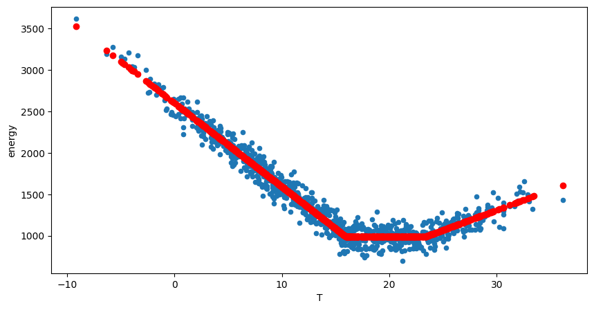
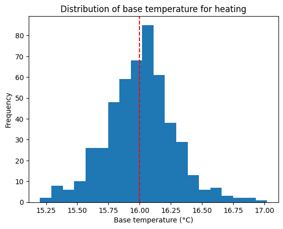
Accessing the performance of the calibration#
The performance of the calibration is assessed by the obtained value with respect to the actual reference temperature used to generate the synthetic data.
We recall that the synthetic data is generated using the following formula
[13]:
n_test = 500
results = []
my_synthtisor = DateSynthTSConsumption(
    base_energy=1e3,
    ts_cool=5e1,
    ts_heat=1e2,
    noise_std=1e2,
    t_ref_cool=24,
    t_ref_heat=16,
)
for idx in range(n_test):
    data = my_synthtisor.random_consumption(start="2021-09-01", end=None, size=200)
    ts = ThermoSensitivity(
        energy_data=data["energy"],
        temperature_data=data["T"],
        frequency="1D",
    )
    ts.degree_days_computation_method = "mean"
    tref = ts.calibrate_base_temperature(
        dd_type="heating", t0=13, xatol=1e-2, disp=False
    )
    results.append(tref)
[14]:
fig, ax = plt.subplots()
ax.hist(results, bins=20)
ax.set_xlabel("Base temperature (°C)")
ax.set_ylabel("Frequency")
ax.set_title("Distribution of base temperature for heating")
ax.axvline(
    x=my_synthtisor.t_ref_heat, color="r", linestyle="--", label="True base temperature"
)
[14]:
<matplotlib.lines.Line2D at 0x7e5afb366850>
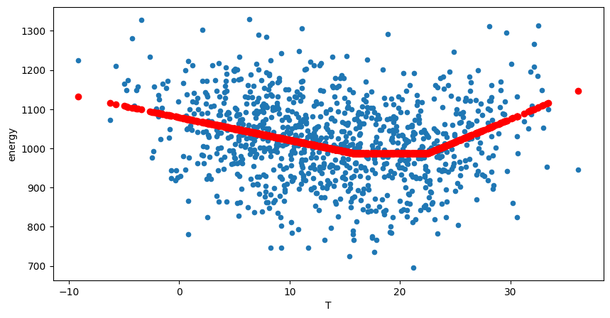
Automatic detection of the type of thermo sensitivity#
In general, it is difficult to know in advance the type of thermo-sensitivity of a building. By “type” I mean : does the building heat during cold days or cool during hot days, or both ?
Hence, it is important to be able to detect it automatically.
By setting the type to "auto", the model will try to detect the type of thermo-sensitivity using Spearman correlation p-value.
[15]:
my_synthtisor_heating = DateSynthTSConsumption(
    base_energy=1e3,
    ts_cool=0,
    ts_heat=1e1,
    noise_std=1e1,
    t_ref_cool=24,
    t_ref_heat=16,
    noise_seed=42,
)

data = my_synthtisor_heating.random_consumption(
    start="2021-09-01", end="2024-04-17", size=None
)

ts = ThermoSensitivity(
    energy_data=data["energy"],
    temperature_data=data["T"],
    frequency="1D",
    degree_days_type="auto",
    degree_days_computation_method="mean",
)
ts.fit()
display(ts.model.summary())

pred = ts.model.predict()

fig, ax = plt.subplots(figsize=(10, 5))
data["energy"].plot(ax=ax, label="Observed")
ax.plot(data.index, pred, label="Predicted")

fig, ax = plt.subplots(figsize=(10, 5))
data.plot.scatter(x="T", y="energy", ax=ax)
ax.scatter(data["T"], ts.model.predict(), label="Predicted", color="r")
| Dep. Variable: | energy | R-squared: | 0.965 |
|---|---|---|---|
| Model: | OLS | Adj. R-squared: | 0.965 |
| Method: | Least Squares | F-statistic: | 1.328e+04 |
| Date: | Fri, 11 Oct 2024 | Prob (F-statistic): | 0.00 |
| Time: | 20:46:28 | Log-Likelihood: | -3583.2 |
| No. Observations: | 960 | AIC: | 7172. |
| Df Residuals: | 957 | BIC: | 7187. |
| Df Model: | 2 | ||
| Covariance Type: | nonrobust |
| coef | std err | t | P>|t| | [0.025 | 0.975] | |
|---|---|---|---|---|---|---|
| heating_degree_days | 10.0768 | 0.065 | 155.803 | 0.000 | 9.950 | 10.204 |
| cooling_degree_days | 0.3656 | 0.177 | 2.063 | 0.039 | 0.018 | 0.713 |
| Intercept | 998.9269 | 0.481 | 2076.770 | 0.000 | 997.983 | 999.871 |
| Omnibus: | 1.366 | Durbin-Watson: | 1.998 |
|---|---|---|---|
| Prob(Omnibus): | 0.505 | Jarque-Bera (JB): | 1.415 |
| Skew: | -0.089 | Prob(JB): | 0.493 |
| Kurtosis: | 2.942 | Cond. No. | 10.6 |
Notes:
[1] Standard Errors assume that the covariance matrix of the errors is correctly specified.
[15]:
<matplotlib.collections.PathCollection at 0x7e5afa822250>
[16]:
my_synthtisor_cooling = DateSynthTSConsumption(
    base_energy=1e3,
    ts_cool=1e1,
    ts_heat=0,
    noise_std=1e2,
    t_ref_cool=24,
    t_ref_heat=16,
)

data = my_synthtisor_cooling.random_consumption(
    start="2021-09-01", end="2024-04-17", size=None
)

ts = ThermoSensitivity(
    energy_data=data["energy"],
    temperature_data=data["T"],
    frequency="1D",
    degree_days_type="auto",
    degree_days_computation_method="mean",
)
ts.fit()
display(ts.model.summary())

pred = ts.model.predict()

fig, ax = plt.subplots(figsize=(10, 5))
data["energy"].plot(ax=ax, label="Observed")
ax.plot(data.index, pred, label="Predicted")

fig, ax = plt.subplots(figsize=(10, 5))
data.plot.scatter(x="T", y="energy", ax=ax)
ax.scatter(data["T"], ts.model.predict(), label="Predicted", color="r")
| Dep. Variable: | energy | R-squared: | 0.041 |
|---|---|---|---|
| Model: | OLS | Adj. R-squared: | 0.040 |
| Method: | Least Squares | F-statistic: | 40.55 |
| Date: | Fri, 11 Oct 2024 | Prob (F-statistic): | 2.97e-10 |
| Time: | 20:46:28 | Log-Likelihood: | -5793.5 |
| No. Observations: | 960 | AIC: | 1.159e+04 |
| Df Residuals: | 958 | BIC: | 1.160e+04 |
| Df Model: | 1 | ||
| Covariance Type: | nonrobust |
| coef | std err | t | P>|t| | [0.025 | 0.975] | |
|---|---|---|---|---|---|---|
| cooling_degree_days | 11.1431 | 1.750 | 6.368 | 0.000 | 7.709 | 14.577 |
| Intercept | 990.8276 | 3.456 | 286.736 | 0.000 | 984.046 | 997.609 |
| Omnibus: | 1.330 | Durbin-Watson: | 1.990 |
|---|---|---|---|
| Prob(Omnibus): | 0.514 | Jarque-Bera (JB): | 1.393 |
| Skew: | -0.086 | Prob(JB): | 0.498 |
| Kurtosis: | 2.928 | Cond. No. | 2.16 |
Notes:
[1] Standard Errors assume that the covariance matrix of the errors is correctly specified.
[16]:
<matplotlib.collections.PathCollection at 0x7e5afa9acf50>
[17]:
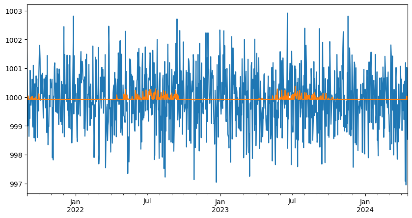
my_synthtisor_both = DateSynthTSConsumption(
    base_energy=1e3,
    ts_cool=1e1,
    ts_heat=5e0,
    noise_std=1e2,
    t_ref_cool=24,
    t_ref_heat=16,
)

data = my_synthtisor_both.random_consumption(start="2021-09-01", end="2024-04-17", size=None)

ts = ThermoSensitivity(
    energy_data=data["energy"],
    temperature_data=data["T"],
    frequency="1D",
    degree_days_type="auto",
    degree_days_computation_method="mean",
)
ts.fit()
display(ts.model.summary())

pred = ts.model.predict()

fig, ax = plt.subplots(figsize=(10, 5))
data["energy"].plot(ax=ax, label="Observed")
ax.plot(data.index, pred, label="Predicted")

fig, ax = plt.subplots(figsize=(10, 5))
data.plot.scatter(x="T", y="energy", ax=ax)
ax.scatter(data["T"], ts.model.predict(), label="Predicted", color="r");
| Dep. Variable: | energy | R-squared: | 0.090 |
|---|---|---|---|
| Model: | OLS | Adj. R-squared: | 0.088 |
| Method: | Least Squares | F-statistic: | 47.26 |
| Date: | Fri, 11 Oct 2024 | Prob (F-statistic): | 2.67e-20 |
| Time: | 20:46:29 | Log-Likelihood: | -5792.9 |
| No. Observations: | 960 | AIC: | 1.159e+04 |
| Df Residuals: | 957 | BIC: | 1.161e+04 |
| Df Model: | 2 | ||
| Covariance Type: | nonrobust |
| coef | std err | t | P>|t| | [0.025 | 0.975] | |
|---|---|---|---|---|---|---|
| heating_degree_days | 5.7894 | 0.651 | 8.889 | 0.000 | 4.511 | 7.067 |
| cooling_degree_days | 11.6883 | 1.831 | 6.383 | 0.000 | 8.095 | 15.282 |
| Intercept | 987.5312 | 4.754 | 207.732 | 0.000 | 978.202 | 996.860 |
| Omnibus: | 1.281 | Durbin-Watson: | 1.997 |
|---|---|---|---|
| Prob(Omnibus): | 0.527 | Jarque-Bera (JB): | 1.339 |
| Skew: | -0.085 | Prob(JB): | 0.512 |
| Kurtosis: | 2.935 | Cond. No. | 10.3 |
Notes:
[1] Standard Errors assume that the covariance matrix of the errors is correctly specified.
[18]:
my_synthtisor_both = DateSynthTSConsumption(
    base_energy=1e3,
    ts_cool=0,
    ts_heat=0,
    noise_std=1e0,
    t_ref_cool=24,
    t_ref_heat=16,
)

data = my_synthtisor_both.random_consumption(start="2021-09-01", end="2024-04-17", size=None)

ts = ThermoSensitivity(
    energy_data=data["energy"],
    temperature_data=data["T"],
    frequency="1D",
    degree_days_type="auto",
    degree_days_computation_method="mean",
)
ts.fit()
display(ts.model.summary())

pred = ts.model.predict()

fig, ax = plt.subplots(figsize=(10, 5))
data["energy"].plot(ax=ax, label="Observed")
ax.plot(data.index, pred, label="Predicted")

fig, ax = plt.subplots(figsize=(10, 5))
data.plot.scatter(x="T", y="energy", ax=ax)
ax.scatter(data["T"], ts.model.predict(), label="Predicted", color="r");
| Dep. Variable: | energy | R-squared: | 0.004 |
|---|---|---|---|
| Model: | OLS | Adj. R-squared: | 0.003 |
| Method: | Least Squares | F-statistic: | 3.827 |
| Date: | Fri, 11 Oct 2024 | Prob (F-statistic): | 0.0507 |
| Time: | 20:46:29 | Log-Likelihood: | -1373.1 |
| No. Observations: | 960 | AIC: | 2750. |
| Df Residuals: | 958 | BIC: | 2760. |
| Df Model: | 1 | ||
| Covariance Type: | nonrobust |
| coef | std err | t | P>|t| | [0.025 | 0.975] | |
|---|---|---|---|---|---|---|
| cooling_degree_days | 0.0330 | 0.017 | 1.956 | 0.051 | -0.000 | 0.066 |
| Intercept | 999.9146 | 0.035 | 2.88e+04 | 0.000 | 999.847 | 999.983 |
| Omnibus: | 1.427 | Durbin-Watson: | 1.992 |
|---|---|---|---|
| Prob(Omnibus): | 0.490 | Jarque-Bera (JB): | 1.483 |
| Skew: | -0.091 | Prob(JB): | 0.476 |
| Kurtosis: | 2.935 | Cond. No. | 2.25 |
Notes:
[1] Standard Errors assume that the covariance matrix of the errors is correctly specified.
[19]:
ts
[19]:
ThermoSensitivity(frequency=1D,
        degree_days_type=cooling,
        degree_days_base_temperature={'heating': np.float64(15.8), 'cooling': np.float64(22.29)},
        degree_days_computation_method=mean,
        interseason_mean_temperature=20)

                            OLS Regression Results
==============================================================================
Dep. Variable:                 energy   R-squared:                       0.004
Model:                            OLS   Adj. R-squared:                  0.003
No. Observations:                 960   F-statistic:                     3.827
Covariance Type:            nonrobust   Prob (F-statistic):             0.0507
=======================================================================================
                          coef    std err          t      P>|t|      [0.025      0.975]
---------------------------------------------------------------------------------------
cooling_degree_days     0.0330      0.017      1.956      0.051      -0.000       0.066
Intercept             999.9146      0.035   2.88e+04      0.000     999.847     999.983
=======================================================================================

Notes:
[1] Standard Errors assume that the covariance matrix of the errors is correctly specified.
Conclusion#
We showed in the notebook how to calibrate the degree days reference temperatures and the thermo-sensitivity model using the synthetic data.
We showed that the calibration is possible and that the performance is reasonable.
Implemented features#
automatic detection of the type of thermo-sensitivity (Heating, Cooling, Mixed), even in the presence of noise.
automatic calibration of the degree days reference temperature (heating and cooling)
automatic calibration of the thermo-sensitivity model (heating and cooling)
Discussion#
To continue the analysis, we could study the impact of the noise level on the calibration performance, usually named Uncertainty Quantification (UQ).
Most of the calibration uses a “intersaison mean temperature” to split the data into heating and cooling periods. By default this value of \(20^\circ C\). It would be interesting to study the impact of this value on the calibration performance.
Categorical thermo-sensitivity#
One of the difficulties of the thermo-sensitivity analysis is the fact that the building behavior can change depending on the day µ(open/closed, week/weekend, holiday, etc).
The following example shows how to use the categorical thermo-sensitivity to model the behavior of a building depending on the day of the week.
[20]:
from energy_analysis_toolbox.synthetic.thermosensitive_consumption import WeekEndSynthTSConsumption

parameters = [
    {
        "base_energy": 1e3,
        "ts_heat": 5e1,
        "ts_cool": 1e2,
        "noise_std": 1e2,
    },
    {
        "base_energy": 1.5e3,
        "ts_heat": 1e1,
        "ts_cool": 6e1,
        "noise_std": 1e2,
    },
]


def open_close_categoriser(series: pd.Series):
    """Return a series of categories based on the day of the week of the index"""
    timestamps = series.index
    return_data = pd.Series(
        data=[
            "Open" if timestamp.weekday() < 5 else "Closed" for timestamp in timestamps
        ],
        index=series.index,
    )
    return return_data


my_cat_synthtisor = WeekEndSynthTSConsumption(
    parameters=parameters,
    t_ref_cool=24,
    t_ref_heat=16,
)
data = my_cat_synthtisor.random_consumption(start="2021-09-01", end="2024-04-17", size=None)
data.head()
[20]:
| base | thermosensitive | residual | energy | heating | cooling | T | DD_heating | DD_cooling | category | |
|---|---|---|---|---|---|---|---|---|---|---|
| 2021-09-01 | 1500.0 | 0.000000 | 30.471708 | 1530.471708 | 0.000000 | 0.000000 | 23.224711 | 0.000000 | 0.000000 | weekday |
| 2021-09-02 | 1500.0 | 0.000000 | -103.998411 | 1396.001589 | 0.000000 | 0.000000 | 16.387722 | 0.000000 | 0.000000 | weekday |
| 2021-09-03 | 1500.0 | 73.467824 | 75.045120 | 1648.512944 | 0.000000 | 73.467824 | 25.224464 | 0.000000 | 1.224464 | weekday |
| 2021-09-04 | 1000.0 | 205.767853 | 30.471708 | 1236.239561 | 0.000000 | 205.767853 | 26.057679 | 0.000000 | 2.057679 | weekend |
| 2021-09-05 | 1000.0 | 225.977849 | -103.998411 | 1121.979438 | 225.977849 | 0.000000 | 11.480443 | 4.519557 | 0.000000 | weekend |
[21]:
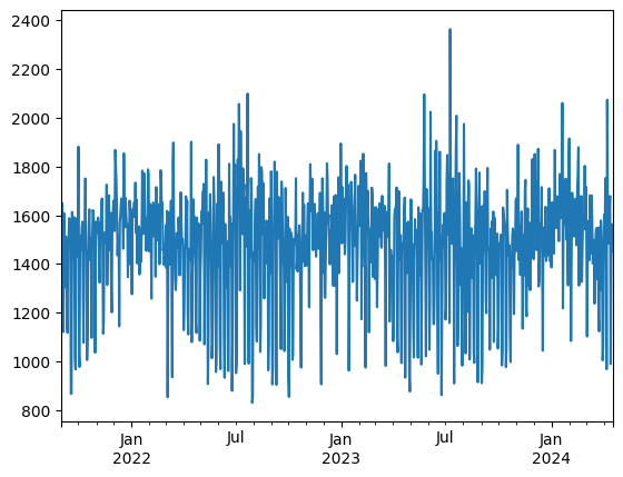
data["energy"].plot();
[22]:
categories = data["category"].unique()
for category in categories:
    subset = data[data["category"] == category]
    plt.scatter(
        subset["T"],
        subset["energy"],
        label=category
    )
plt.xlabel("T")
plt.ylabel("energy")
plt.legend(title="category")
plt.show()
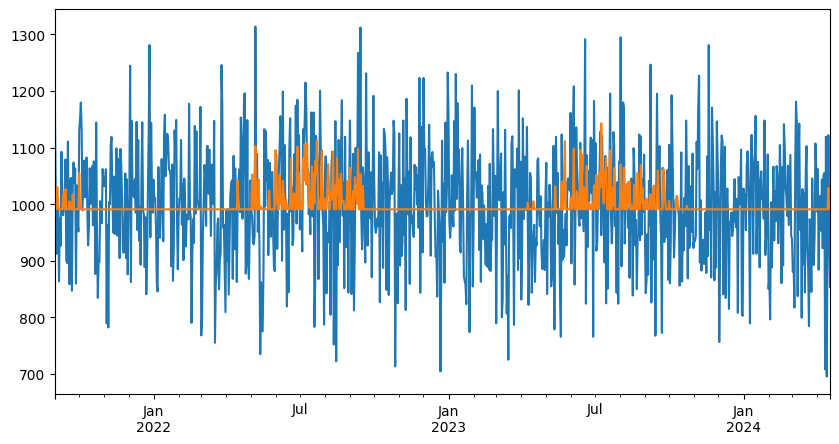
Using no category#
As a first step, we can consider that the building has no category and that the behavior is the same every day.
[23]:
ts_no_cat = ThermoSensitivity(
    energy_data=data["energy"],
    temperature_data=data["T"],
    frequency="1D",
    degree_days_type="auto",
    degree_days_computation_method="mean",
)
ts_no_cat.fit()
# display(ts_no_cat.model.summary())
fig, [ax1, ax2] = plt.subplots(1, 2, figsize=(10, 5))
ax1.scatter(data["T"], data["energy"], label="Observed")
ax1.scatter(data["T"], ts_no_cat.model.predict(), label="Predicted", color="r")
ax1.legend()

error = data["energy"] - ts_no_cat.model.predict()
error = pd.concat([error, data["category"]], axis=1)

categories = data["category"].unique()

for category in categories:
    subset = data[data["category"] == category]
    ax2.hist(
        subset["energy"],
        bins=30,
        alpha=0.6,
        label=category,
        density=False,
    )
ax2.set_xlabel("energy")
ax2.set_ylabel('Frequency')
ax2.legend(title="category");
Using Categories#
Now, lets consider that the building has two categories: week and weekend (fortunately, we know how the data is generated).
[24]:
categories = open_close_categoriser(data).rename("category")
categories
[24]:
2021-09-01      Open
2021-09-02      Open
2021-09-03      Open
2021-09-04    Closed
2021-09-05    Closed
               ...
2024-04-13    Closed
2024-04-14    Closed
2024-04-15      Open
2024-04-16      Open
2024-04-17      Open
Name: category, Length: 960, dtype: object
[25]:
from energy_analysis_toolbox.thermosensitivity.thermosensitivity import (
    CategoricalThermoSensitivity,
)

ts_cat = CategoricalThermoSensitivity(
    energy_data=data["energy"],
    temperature_data=data["T"],
    categories=categories,
    frequency="1D",
    degree_days_type="auto",
    degree_days_computation_method="mean",
)
ts_cat.fit()
[25]:
CategoricalThermoSensitivity(frequency=1D,
        degree_days_type=both,
        degree_days_base_temperature={'heating': np.float64(14.37), 'cooling': np.float64(23.82)},
        degree_days_computation_method=mean,
        interseason_mean_temperature=20)

                            OLS Regression Results
==============================================================================
Dep. Variable:                 energy   R-squared:                       0.814
Model:                            OLS   Adj. R-squared:                  0.813
No. Observations:                 960   F-statistic:                     834.1
Covariance Type:            nonrobust   Prob (F-statistic):               0.00
==============================================================================================
                                 coef    std err          t      P>|t|      [0.025      0.975]
----------------------------------------------------------------------------------------------
heating_degree_days:Closed    55.4922      1.360     40.816      0.000      52.824      58.160
heating_degree_days:Open      10.7250      0.797     13.454      0.000       9.161      12.289
cooling_degree_days:Closed    93.9007      3.979     23.601      0.000      86.093     101.709
cooling_degree_days:Open      54.1264      2.563     21.118      0.000      49.096      59.156
Intercept:Closed            1025.8751      8.237    124.546      0.000    1009.711    1042.040
Intercept:Open              1504.6139      5.049    297.985      0.000    1494.705    1514.523
==============================================================================================

Notes:
[1] Standard Errors assume that the covariance matrix of the errors is correctly specified.
[26]:
ts_cat.model.summary()
[26]:
| Dep. Variable: | energy | R-squared: | 0.814 |
|---|---|---|---|
| Model: | OLS | Adj. R-squared: | 0.813 |
| Method: | Least Squares | F-statistic: | 834.1 |
| Date: | Fri, 11 Oct 2024 | Prob (F-statistic): | 0.00 |
| Time: | 20:46:30 | Log-Likelihood: | -5762.8 |
| No. Observations: | 960 | AIC: | 1.154e+04 |
| Df Residuals: | 954 | BIC: | 1.157e+04 |
| Df Model: | 5 | ||
| Covariance Type: | nonrobust |
| coef | std err | t | P>|t| | [0.025 | 0.975] | |
|---|---|---|---|---|---|---|
| heating_degree_days:Closed | 55.4922 | 1.360 | 40.816 | 0.000 | 52.824 | 58.160 |
| heating_degree_days:Open | 10.7250 | 0.797 | 13.454 | 0.000 | 9.161 | 12.289 |
| cooling_degree_days:Closed | 93.9007 | 3.979 | 23.601 | 0.000 | 86.093 | 101.709 |
| cooling_degree_days:Open | 54.1264 | 2.563 | 21.118 | 0.000 | 49.096 | 59.156 |
| Intercept:Closed | 1025.8751 | 8.237 | 124.546 | 0.000 | 1009.711 | 1042.040 |
| Intercept:Open | 1504.6139 | 5.049 | 297.985 | 0.000 | 1494.705 | 1514.523 |
| Omnibus: | 3.208 | Durbin-Watson: | 1.925 |
|---|---|---|---|
| Prob(Omnibus): | 0.201 | Jarque-Bera (JB): | 3.150 |
| Skew: | 0.140 | Prob(JB): | 0.207 |
| Kurtosis: | 3.018 | Cond. No. | 13.7 |
Notes:
[1] Standard Errors assume that the covariance matrix of the errors is correctly specified.
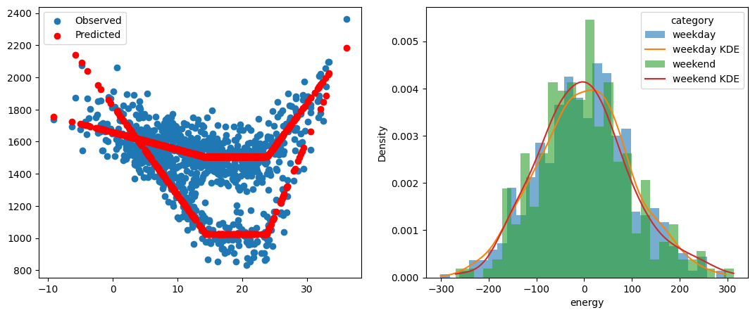
[27]:
from scipy.stats import gaussian_kde
import numpy as np

fig, [ax1, ax2] = plt.subplots(1, 2, figsize=(13, 5))
ax1.scatter(data["T"], data["energy"], label="Observed")
ax1.scatter(data["T"], ts_cat.model.predict(), label="Predicted", color="r")
ax1.legend()

error = data["energy"] - ts_cat.model.predict()
error = pd.concat([error, data["category"]], axis=1)

categories = error["category"].unique()

for category in categories:
    subset = error[error["category"] == category]
    ax2.hist(
        subset["energy"],
        bins=30,
        alpha=0.6,
        label=category,
        density=True
    )
    kde_data = gaussian_kde(subset["energy"])
    x_vals = np.linspace(subset["energy"].min(), subset["energy"].max(), 100)
    ax2.plot(x_vals, kde_data(x_vals), label=f'{category} KDE')

ax2.set_xlabel("energy")
ax2.set_ylabel("Density")
ax2.legend(title="category");
Automatic detection of the category to use#
[28]:
from energy_analysis_toolbox.thermosensitivity.daily_analysis import (
    AutoCategoricalThermoSensitivity,
)
[29]:
data = data = my_cat_synthtisor.random_consumption(
    start="2021-09-01", end="2024-04-17", size=None
)


ts = AutoCategoricalThermoSensitivity(
    energy_data=data["energy"],
    temperature_data=data["T"],
    degree_days_type="auto",
    degree_days_computation_method="mean",
)

ts.fit()
[29]:
AutoCategoricalThermoSensitivity(frequency=1D,
        degree_days_type=both,
        degree_days_base_temperature={'heating': np.float64(17.69), 'cooling': np.float64(23.78)},
        degree_days_computation_method=mean,
        interseason_mean_temperature=20)

                            OLS Regression Results
==============================================================================
Dep. Variable:                 energy   R-squared:                       0.818
Model:                            OLS   Adj. R-squared:                  0.814
No. Observations:                 960   F-statistic:                     211.0
Covariance Type:            nonrobust   Prob (F-statistic):               0.00
=================================================================================================
                                    coef    std err          t      P>|t|      [0.025      0.975]
-------------------------------------------------------------------------------------------------
heating_degree_days:Friday       11.3549      1.618      7.018      0.000       8.180      14.530
heating_degree_days:Monday       10.7842      1.627      6.628      0.000       7.591      13.977
heating_degree_days:Saturday     47.0777      1.514     31.091      0.000      44.106      50.049
heating_degree_days:Sunday       44.8014      1.566     28.612      0.000      41.728      47.874
heating_degree_days:Thursday      9.6483      1.414      6.824      0.000       6.873      12.423
heating_degree_days:Tuesday      12.6799      1.610      7.874      0.000       9.520      15.840
heating_degree_days:Wednesday     8.9878      1.590      5.652      0.000       5.867      12.109
cooling_degree_days:Friday       52.4540      5.293      9.909      0.000      42.066      62.842
cooling_degree_days:Monday       64.9016      5.056     12.836      0.000      54.979      74.824
cooling_degree_days:Saturday    106.9762      6.504     16.448      0.000      94.213     119.740
cooling_degree_days:Sunday      103.4060      6.111     16.922      0.000      91.414     115.398
cooling_degree_days:Thursday     46.1212      8.220      5.611      0.000      29.990      62.252
cooling_degree_days:Tuesday      67.4154      7.078      9.525      0.000      53.525      81.306
cooling_degree_days:Wednesday    58.3910      5.192     11.245      0.000      48.201      68.581
Intercept:Friday               1487.4244     13.753    108.156      0.000    1460.435    1514.414
Intercept:Monday               1462.3171     13.209    110.702      0.000    1436.394    1488.241
Intercept:Saturday              960.5433     12.962     74.105      0.000     935.106     985.981
Intercept:Sunday                970.0862     13.328     72.785      0.000     943.930     996.243
Intercept:Thursday             1492.6268     13.229    112.827      0.000    1466.664    1518.589
Intercept:Tuesday              1479.5532     12.869    114.973      0.000    1454.298    1504.808
Intercept:Wednesday            1491.0792     13.386    111.394      0.000    1464.810    1517.348
=================================================================================================

Notes:
[1] Standard Errors assume that the covariance matrix of the errors is correctly specified.
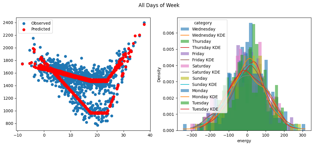
[30]:
fig, [ax1, ax2] = plt.subplots(1, 2, figsize=(13, 5))
ax1.scatter(ts.resampled_temperature, ts.resampled_energy, label="Observed")
ax1.scatter(ts.resampled_temperature, ts.model.predict(), label="Predicted", color="r")
ax1.legend()

error = ts.resampled_energy - ts.model.predict()
error = pd.concat([error, ts.resampled_categories], axis=1)

categories = error["category"].unique()

for category in categories:
    subset = error[error["category"] == category]
    ax2.hist(
        subset["energy"],
        bins=30,
        alpha=0.6,
        label=category,
        density=True
    )
    kde_data = gaussian_kde(subset["energy"])
    x_vals = np.linspace(subset["energy"].min(), subset["energy"].max(), 100)
    ax2.plot(x_vals, kde_data(x_vals), label=f'{category} KDE')

ax2.set_xlabel("energy")
ax2.set_ylabel("Density")
ax2.legend(title="category")

fig.suptitle("All Days of Week");
[31]:
ts.merge_and_fit()
[32]:
fig, [ax1, ax2] = plt.subplots(1, 2, figsize=(13, 5))
ax1.scatter(ts.resampled_temperature, ts.resampled_energy, label="Observed")
ax1.scatter(ts.resampled_temperature, ts.model.predict(), label="Predicted", color="r")
ax1.legend()

error = ts.resampled_energy - ts.model.predict()
error = pd.concat([error, ts.resampled_categories], axis=1)
categories = error["category"].unique()

for category in categories:
    subset = error[error["category"] == category]
    ax2.hist(
        subset["energy"],
        bins=30,
        alpha=0.6,
        label=category,
        density=True
    )

    # KDE
    kde_data = gaussian_kde(subset["energy"])
    x_vals = np.linspace(subset["energy"].min(), subset["energy"].max(), 100)
    ax2.plot(x_vals, kde_data(x_vals), label=f'{category} KDE')

ax2.set_xlabel("energy")
ax2.set_ylabel("Density")
ax2.legend(title="category")
fig.suptitle("After Merging of Similar Categories");
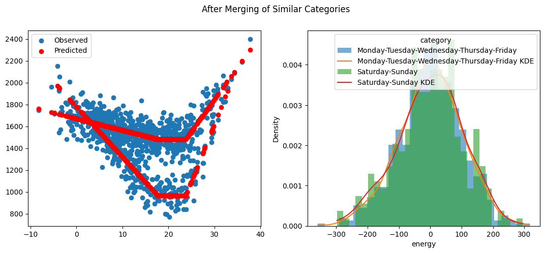
As expected, the days with the same categories are similare. Lets see if the model can capture the difference between the days.
Conclusion#
We have seen how we can analyse the consumption of a building depending even with different thermo-sensitivity depending on the day.
However, we still need to see how the model behaves in the presence of labeling errors. Typically, we could have a day that is labeled as a weekend day but that is actually with a week day behavior.