Using eat for thermosensitivity analysis: Real data#
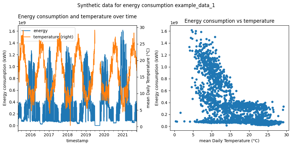
This notebook uses data from the real world. It comes from a school building. Hence, it shows a large variety of occupancy:
usual school days
usual weekends
Wednesdays can differ from the other days
Bank holidays
school holidays either closed, or with another occupancy (think of a summer camp)
[1]:
import matplotlib.pyplot as plt
import pandas as pd
import seaborn as sns
[2]:
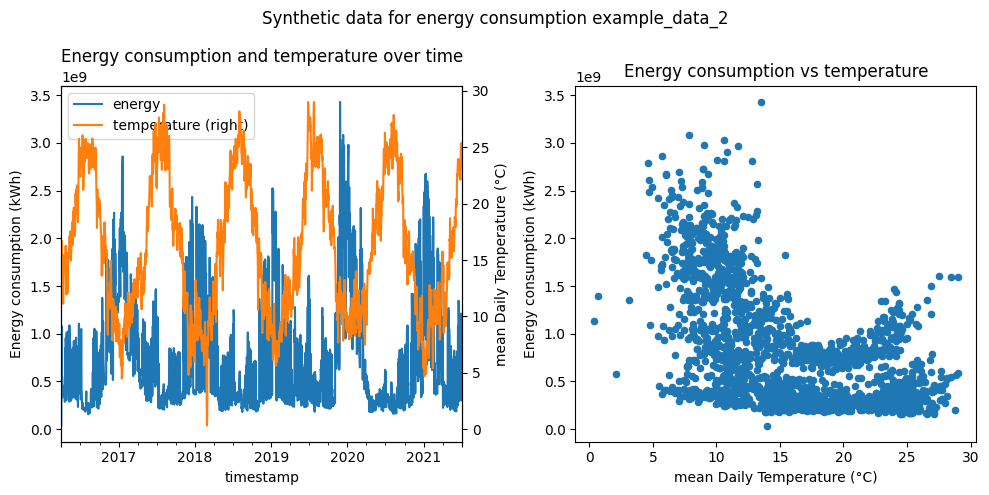
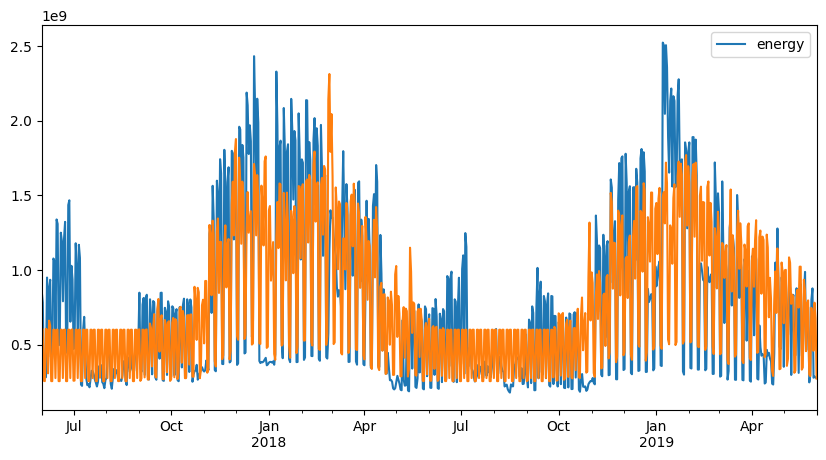
files = ["data/example_data_1.parquet", "data/example_data_2.parquet"]

for file in files:
    data = pd.read_parquet(file)
    data = data.resample("1D").agg({"energy": "sum", "temperature": "mean"})
    fig, [ax1, ax2] = plt.subplots(1, 2, figsize=(10, 5))
    data[["energy"]].plot(ax=ax1)
    data[["temperature"]].plot(ax=ax1, secondary_y=True)
    ax1.set_ylabel("Energy consumption (kWh)")
    ax1.right_ax.set_ylabel("mean Daily Temperature (°C)")
    data.plot.scatter(x="temperature", y="energy", ax=ax2)
    ax2.set_xlabel("mean Daily Temperature (°C)")
    ax2.set_ylabel("Energy consumption (kWh)")
    ax1.set_title("Energy consumption and temperature over time")
    ax2.set_title("Energy consumption vs temperature")
    fig.suptitle(
        "Synthetic data for energy consumption " + file.split("/")[-1].split(".")[0]
    )
    fig.tight_layout()
Thermo-sensitivity analysis#
The main objective of the analysis is to explain the impact of the temperature over the energy.
Each category of occupancy can be modeled with a thermosensitivity model by: - finding the threshold temperatures for heating and cooling - finding the three coefficients \(E_0\), \(TS_{cooling}\) and \(TS_{heating}\) such that
But this must be done for all the different (unlabeled) categories.
Modeling the Weekly energy#
The first step is to model the weekly energy consumption. This is done by passing the frequencu “7D” to the ThermoSensitivity class.
Processing weekly data is a good way to get a first idea of the thermosensitivity of the building without being too much influenced by the daily variations.
[3]:
from energy_analysis_toolbox.thermosensitivity import ThermoSensitivity
[4]:
data = pd.read_parquet(files[0])
start = data.index[0]
first_monday = start + pd.DateOffset(weekday=0, hour=0, minute=0, second=0)
data = data.loc[first_monday:]
data.head()
[4]:
| duration | energy | holidays | temperature | |
|---|---|---|---|---|
| timestamp | ||||
| 2015-05-04 00:00:00+02:00 | 600000.0 | 600000.0 | True | 15.800000 |
| 2015-05-04 00:10:00+02:00 | 600000.0 | 1200000.0 | True | 15.766667 |
| 2015-05-04 00:20:00+02:00 | 600000.0 | 1200000.0 | True | 15.733333 |
| 2015-05-04 00:30:00+02:00 | 600000.0 | 1200000.0 | True | 15.700000 |
| 2015-05-04 00:40:00+02:00 | 600000.0 | 600000.0 | True | 15.666667 |
[5]:
ts = ThermoSensitivity(
    energy_data=data["energy"],
    temperature_data=data["temperature"],
    frequency="7D",
    degree_days_type="auto",
    degree_days_computation_method="integral",
)
[6]:
ts.fit()
ts.model.summary()
[6]:
| Dep. Variable: | energy | R-squared: | 0.568 |
|---|---|---|---|
| Model: | OLS | Adj. R-squared: | 0.566 |
| Method: | Least Squares | F-statistic: | 421.2 |
| Date: | Fri, 11 Oct 2024 | Prob (F-statistic): | 2.21e-60 |
| Time: | 20:44:14 | Log-Likelihood: | -7243.9 |
| No. Observations: | 323 | AIC: | 1.449e+04 |
| Df Residuals: | 321 | BIC: | 1.450e+04 |
| Df Model: | 1 | ||
| Covariance Type: | nonrobust |
| coef | std err | t | P>|t| | [0.025 | 0.975] | |
|---|---|---|---|---|---|---|
| heating_degree_days | 6.991e+07 | 3.41e+06 | 20.523 | 0.000 | 6.32e+07 | 7.66e+07 |
| Intercept | 1.089e+09 | 1.01e+08 | 10.746 | 0.000 | 8.9e+08 | 1.29e+09 |
| Omnibus: | 46.497 | Durbin-Watson: | 0.965 |
|---|---|---|---|
| Prob(Omnibus): | 0.000 | Jarque-Bera (JB): | 130.523 |
| Skew: | -0.649 | Prob(JB): | 4.54e-29 |
| Kurtosis: | 5.831 | Cond. No. | 40.7 |
Notes:
[1] Standard Errors assume that the covariance matrix of the errors is correctly specified.
[7]:
ts.aggregated_data
[7]:
| energy | temperature | heating_degree_days | |
|---|---|---|---|
| timestamp | |||
| 2015-05-04 00:00:00+02:00 | 8.418000e+08 | 18.067510 | 2.365944 |
| 2015-05-11 00:00:00+02:00 | 1.519200e+09 | 19.319345 | 1.547856 |
| 2015-05-18 00:00:00+02:00 | 1.975200e+09 | 17.227480 | 4.530394 |
| 2015-05-25 00:00:00+02:00 | 1.726800e+09 | 17.525794 | 2.079876 |
| 2015-06-01 00:00:00+02:00 | 1.925400e+09 | 22.076042 | 0.111308 |
| ... | ... | ... | ... |
| 2021-09-06 00:00:00+02:00 | 1.674000e+09 | 22.365526 | 0.000000 |
| 2021-09-13 00:00:00+02:00 | 1.678800e+09 | 21.557242 | 0.000000 |
| 2021-09-20 00:00:00+02:00 | 1.786200e+09 | 19.917758 | 0.473862 |
| 2021-09-27 00:00:00+02:00 | 1.790400e+09 | 19.841270 | 0.058568 |
| 2021-10-04 00:00:00+02:00 | 1.202400e+09 | 17.835594 | 0.995487 |
336 rows × 3 columns
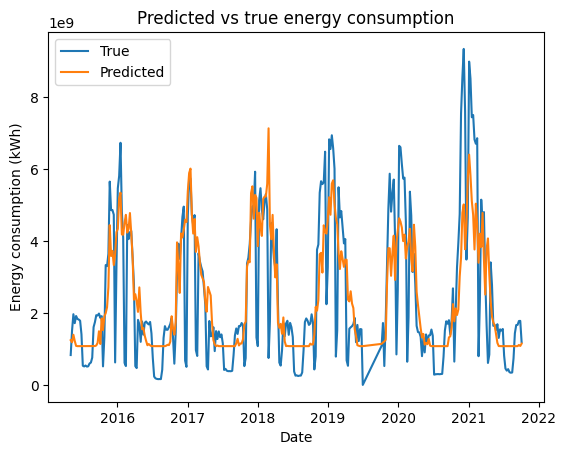
[8]:
predictions = ts.model.predict()

fig, ax = plt.subplots()
aggregated_data = ts.aggregated_data.dropna(how="any", axis=0)
ax.plot(aggregated_data.index, aggregated_data["energy"], label="True")
ax.plot(aggregated_data.index, predictions, label="Predicted")
ax.legend()
ax.set_title("Predicted vs true energy consumption")
ax.set_ylabel("Energy consumption (kWh)")
ax.set_xlabel("Date")
[8]:
Text(0.5, 0, 'Date')
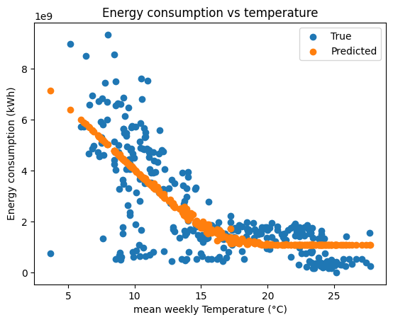
[9]:
fig, ax = plt.subplots()

ax.scatter(aggregated_data["temperature"], aggregated_data["energy"], label="True")
ax.scatter(aggregated_data["temperature"], predictions, label="Predicted")
ax.legend()
ax.set_xlabel("mean weekly Temperature (°C)")
ax.set_ylabel("Energy consumption (kWh)")
ax.set_title("Energy consumption vs temperature")
[9]:
Text(0.5, 1.0, 'Energy consumption vs temperature')
[10]:
data2 = pd.read_parquet(files[1])
start = data2.index[0]
first_monday = start + pd.DateOffset(weekday=0, hour=0, minute=0, second=0)
data2 = data2.loc[first_monday:]
ts2 = ThermoSensitivity(
    energy_data=data2["energy"],
    temperature_data=data2["temperature"],
    frequency="7D",
    degree_days_type="auto",
    degree_days_computation_method="integral",  # here the provided data is already in daily frequency. Hence the only mean
)
ts2.fit()
predictions2 = ts2.model.predict()

fig, ax = plt.subplots()
aggregated_data = ts2.aggregated_data.dropna(how="any", axis=0)
ax.plot(aggregated_data.index, aggregated_data["energy"], label="True")
ax.plot(aggregated_data.index, predictions2, label="Predicted")
ax.legend()
ax.set_title("Predicted vs true energy consumption")
ax.set_ylabel("Energy consumption (kWh)")
ax.set_xlabel("Date")

fig, ax = plt.subplots()
ax.scatter(aggregated_data["temperature"], aggregated_data["energy"], label="True")
ax.scatter(aggregated_data["temperature"], predictions2, label="Predicted")
ax.legend()
ax.set_xlabel("mean weekly Temperature (°C)")
ax.set_ylabel("Energy consumption (kWh)")
ax.set_title("Energy consumption vs temperature")
[10]:
Text(0.5, 1.0, 'Energy consumption vs temperature')
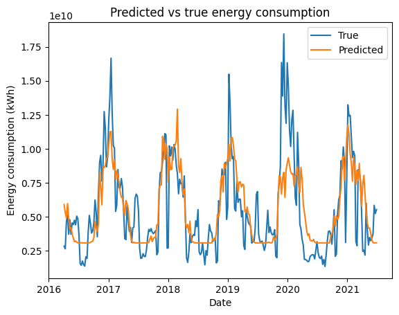
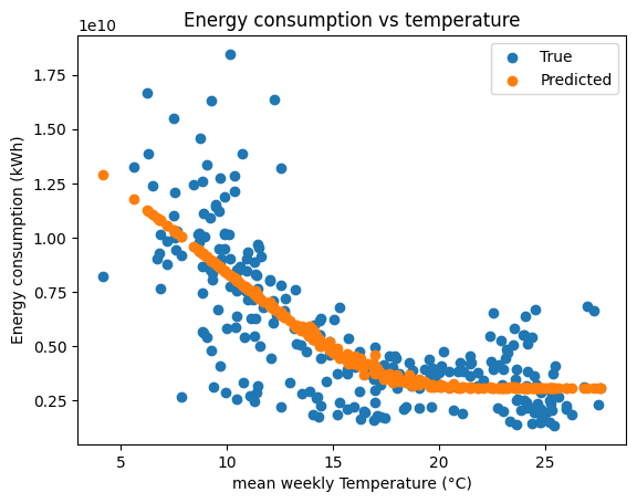
Conclusion of Weekly Analysis#
As you can see above, the model is able to fit the data quite well. The model is able to capture the heating and cooling needs of the building.
One limitation that we can observe is the drop in energy consumption during the summer. This is due to the fact that the building is closed during the summer. This is a limitation of the model as it is not able to capture the occupancy of the building.
Modeling the Daily energy#
The next step is to model the daily energy consumption. This is done by passing the frequency “1D” to the ThermoSensitivity class.
However, the daily data is more complex to model as it is influenced by the occupancy of the building.
[11]:
from energy_analysis_toolbox.thermosensitivity.thermosensitivity import (
CategoricalThermoSensitivity,
)
data = pd.read_parquet(files[0]).loc[
"2016-02-01":"2018-10-01"
] # Selecting dates where the behaviour is more stable
start = data.index[0]
first_monday = start + pd.DateOffset(weekday=0, hour=0, minute=0, second=0)
data = data.loc[first_monday:]
def open_close_categoriser(series: pd.Series):
"""Return a series of categories based on the day of the week of the index"""
timestamps = series.index
return_data = pd.Series(
data=[
"Open" if timestamp.weekday() < 5 else "Closed" for timestamp in timestamps
],
index=series.index,
)
return return_data
categories = open_close_categoriser(data)
display(categories.head())
ts_cat = CategoricalThermoSensitivity(
energy_data=data["energy"],
temperature_data=data["temperature"],
categories=categories,
frequency="1D",
degree_days_type="auto",
degree_days_computation_method="mean",
)
ts_cat.fit()
display(ts_cat.model.summary())
predictions = ts_cat.model.predict()
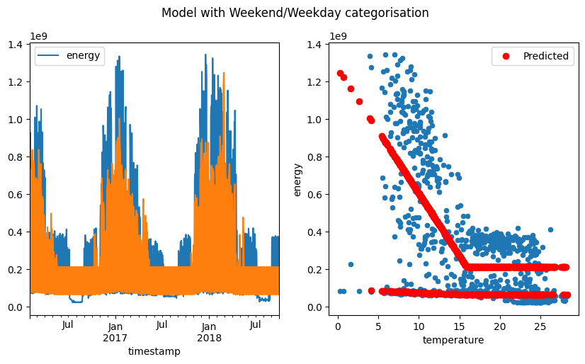
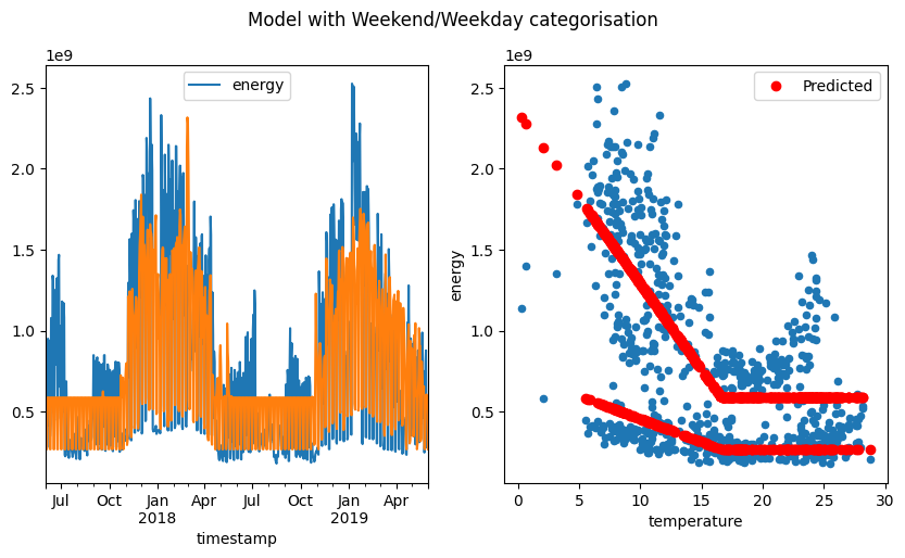
fig, [ax1, ax2] = plt.subplots(1, 2, figsize=(10, 5))
aggregated_data = ts_cat.aggregated_data.dropna(how="any", axis=0)
aggregated_data[["energy"]].plot(ax=ax1)
ax1.plot(aggregated_data.index, predictions, label="Predicted")
aggregated_data.plot.scatter(x="temperature", y="energy", ax=ax2)
ax2.scatter(aggregated_data["temperature"], predictions, label="Predicted", color="red")
ax2.legend()
fig.suptitle("Model with Weekend/Weekday categorisation")
timestamp
2016-02-01 00:00:00+01:00    Open
2016-02-01 00:10:00+01:00    Open
2016-02-01 00:20:00+01:00    Open
2016-02-01 00:30:00+01:00    Open
2016-02-01 00:40:00+01:00    Open
dtype: object
| Dep. Variable: | energy | R-squared: | 0.522 |
|---|---|---|---|
| Model: | OLS | Adj. R-squared: | 0.520 |
| Method: | Least Squares | F-statistic: | 352.9 |
| Date: | Fri, 11 Oct 2024 | Prob (F-statistic): | 6.83e-155 |
| Time: | 20:44:16 | Log-Likelihood: | -20126. |
| No. Observations: | 974 | AIC: | 4.026e+04 |
| Df Residuals: | 970 | BIC: | 4.028e+04 |
| Df Model: | 3 | ||
| Covariance Type: | nonrobust |
| coef | std err | t | P>|t| | [0.025 | 0.975] | |
|---|---|---|---|---|---|---|
| heating_degree_days:Closed | 1.855e+06 | 4.2e+06 | 0.442 | 0.659 | -6.39e+06 | 1.01e+07 |
| heating_degree_days:Open | 6.648e+07 | 2.57e+06 | 25.819 | 0.000 | 6.14e+07 | 7.15e+07 |
| Intercept:Closed | 6.558e+07 | 1.75e+07 | 3.756 | 0.000 | 3.13e+07 | 9.98e+07 |
| Intercept:Open | 2.124e+08 | 1.11e+07 | 19.157 | 0.000 | 1.91e+08 | 2.34e+08 |
| Omnibus: | 124.025 | Durbin-Watson: | 1.065 |
|---|---|---|---|
| Prob(Omnibus): | 0.000 | Jarque-Bera (JB): | 375.035 |
| Skew: | -0.632 | Prob(JB): | 3.65e-82 |
| Kurtosis: | 5.765 | Cond. No. | 8.88 |
Notes:
[1] Standard Errors assume that the covariance matrix of the errors is correctly specified.
[11]:
Text(0.5, 0.98, 'Model with Weekend/Weekday categorisation')
[12]:
data = pd.read_parquet(files[0]).loc[
"2016-02-01":"2018-10-01"
] # Selecting dates where the behaviour is more stable
def dayofweek_categoriser(series: pd.Series):
"""Return a series of categories based on the day of the week of the index"""
timestamps = series.index
return_data = pd.Series(
data=[timestamp.weekday() for timestamp in timestamps],
index=series.index,
)
return return_data
categories = dayofweek_categoriser(data)
display(categories.head())
ts_cat = CategoricalThermoSensitivity(
energy_data=data["energy"],
temperature_data=data["temperature"],
categories=categories,
frequency="1D",
degree_days_type="auto",
degree_days_computation_method="mean",
)
ts_cat.fit()
display(ts_cat.model.summary())
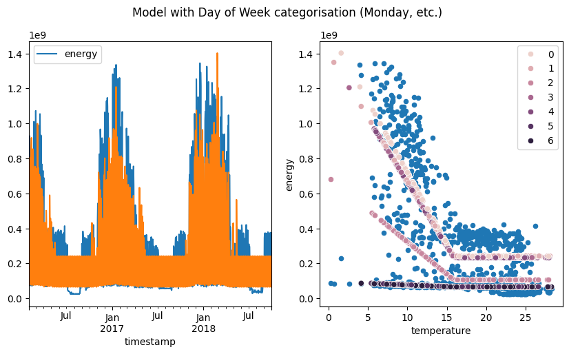
predictions = ts_cat.model.predict()
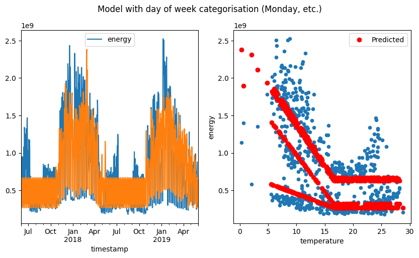
fig, [ax1, ax2] = plt.subplots(1, 2, figsize=(10, 5))
aggregated_data = ts_cat.aggregated_data.dropna(how="any", axis=0)
aggregated_data[["energy"]].plot(ax=ax1)
ax1.plot(aggregated_data.index, predictions, label="Predicted")
aggregated_data.plot.scatter(x="temperature", y="energy", ax=ax2)
sns.scatterplot(
x=aggregated_data["temperature"], y=predictions, hue=aggregated_data["category"]
)
ax2.legend()
fig.suptitle("Model with Day of Week categorisation (Monday, etc.)")
timestamp
2016-02-01 00:00:00+01:00    0
2016-02-01 00:10:00+01:00    0
2016-02-01 00:20:00+01:00    0
2016-02-01 00:30:00+01:00    0
2016-02-01 00:40:00+01:00    0
dtype: int64
| Dep. Variable: | energy | R-squared: | 0.601 |
|---|---|---|---|
| Model: | OLS | Adj. R-squared: | 0.595 |
| Method: | Least Squares | F-statistic: | 111.0 |
| Date: | Fri, 11 Oct 2024 | Prob (F-statistic): | 6.43e-181 |
| Time: | 20:44:16 | Log-Likelihood: | -20039. |
| No. Observations: | 974 | AIC: | 4.011e+04 |
| Df Residuals: | 960 | BIC: | 4.017e+04 |
| Df Model: | 13 | ||
| Covariance Type: | nonrobust |
| coef | std err | t | P>|t| | [0.025 | 0.975] | |
|---|---|---|---|---|---|---|
| heating_degree_days:0.0 | 8.133e+07 | 5.36e+06 | 15.171 | 0.000 | 7.08e+07 | 9.18e+07 |
| heating_degree_days:1.0 | 7.282e+07 | 5.28e+06 | 13.788 | 0.000 | 6.25e+07 | 8.32e+07 |
| heating_degree_days:2.0 | 3.684e+07 | 5.1e+06 | 7.229 | 0.000 | 2.68e+07 | 4.68e+07 |
| heating_degree_days:3.0 | 7.318e+07 | 5.25e+06 | 13.931 | 0.000 | 6.29e+07 | 8.35e+07 |
| heating_degree_days:4.0 | 7.303e+07 | 5.48e+06 | 13.315 | 0.000 | 6.23e+07 | 8.38e+07 |
| heating_degree_days:5.0 | 1.907e+06 | 5.43e+06 | 0.351 | 0.725 | -8.75e+06 | 1.26e+07 |
| heating_degree_days:6.0 | 1.8e+06 | 5.49e+06 | 0.328 | 0.743 | -8.97e+06 | 1.26e+07 |
| Intercept:0.0 | 2.402e+08 | 2.28e+07 | 10.552 | 0.000 | 1.96e+08 | 2.85e+08 |
| Intercept:1.0 | 2.414e+08 | 2.27e+07 | 10.613 | 0.000 | 1.97e+08 | 2.86e+08 |
| Intercept:2.0 | 1.054e+08 | 2.27e+07 | 4.637 | 0.000 | 6.08e+07 | 1.5e+08 |
| Intercept:3.0 | 2.33e+08 | 2.28e+07 | 10.215 | 0.000 | 1.88e+08 | 2.78e+08 |
| Intercept:4.0 | 2.32e+08 | 2.29e+07 | 10.143 | 0.000 | 1.87e+08 | 2.77e+08 |
| Intercept:5.0 | 6.622e+07 | 2.27e+07 | 2.919 | 0.004 | 2.17e+07 | 1.11e+08 |
| Intercept:6.0 | 6.494e+07 | 2.27e+07 | 2.863 | 0.004 | 2.04e+07 | 1.09e+08 |
| Omnibus: | 330.600 | Durbin-Watson: | 0.781 |
|---|---|---|---|
| Prob(Omnibus): | 0.000 | Jarque-Bera (JB): | 1675.453 |
| Skew: | -1.482 | Prob(JB): | 0.00 |
| Kurtosis: | 8.701 | Cond. No. | 5.86 |
Notes:
[1] Standard Errors assume that the covariance matrix of the errors is correctly specified.
[12]:
Text(0.5, 0.98, 'Model with Day of Week categorisation (Monday, etc.)')
[13]:
data2 = pd.read_parquet(files[1]).loc[
    "2017-06-01":"2019-06-01"
]  # Selecting dates where the behaviour is more stable


def open_close_categoriser(series: pd.Series):
    """Return a series of categories based on the day of the week of the index"""
    timestamps = series.index
    return_data = pd.Series(
        data=[
            "Open" if timestamp.weekday() < 5 else "Closed" for timestamp in timestamps
        ],
        index=series.index,
    )
    return return_data


categories = open_close_categoriser(data2)
display(categories.head())

ts_cat = CategoricalThermoSensitivity(
    energy_data=data2["energy"],
    temperature_data=data2["temperature"],
    categories=categories,
    frequency="1D",
    degree_days_type="auto",
    degree_days_computation_method="mean",
)
ts_cat.fit()

display(ts_cat.model.summary())
predictions = ts_cat.model.predict()
fig, [ax1, ax2] = plt.subplots(1, 2, figsize=(10, 5))
aggregated_data = ts_cat.aggregated_data.dropna(how="any", axis=0)
aggregated_data[["energy"]].plot(ax=ax1)
ax1.plot(aggregated_data.index, predictions, label="Predicted")

aggregated_data.plot.scatter(x="temperature", y="energy", ax=ax2)
ax2.scatter(aggregated_data["temperature"], predictions, label="Predicted", color="red")
ax2.legend()
fig.suptitle("Model with Weekend/Weekday categorisation")
timestamp
2017-06-01 00:00:00+02:00    Open
2017-06-01 00:10:00+02:00    Open
2017-06-01 00:20:00+02:00    Open
2017-06-01 00:30:00+02:00    Open
2017-06-01 00:40:00+02:00    Open
dtype: object
| Dep. Variable: | energy | R-squared: | 0.588 |
|---|---|---|---|
| Model: | OLS | Adj. R-squared: | 0.586 |
| Method: | Least Squares | F-statistic: | 346.1 |
| Date: | Fri, 11 Oct 2024 | Prob (F-statistic): | 1.47e-139 |
| Time: | 20:44:17 | Log-Likelihood: | -15439. |
| No. Observations: | 731 | AIC: | 3.089e+04 |
| Df Residuals: | 727 | BIC: | 3.090e+04 |
| Df Model: | 3 | ||
| Covariance Type: | nonrobust |
| coef | std err | t | P>|t| | [0.025 | 0.975] | |
|---|---|---|---|---|---|---|
| heating_degree_days:Closed | 2.833e+07 | 6.95e+06 | 4.078 | 0.000 | 1.47e+07 | 4.2e+07 |
| heating_degree_days:Open | 1.062e+08 | 4.23e+06 | 25.095 | 0.000 | 9.79e+07 | 1.15e+08 |
| Intercept:Closed | 2.67e+08 | 3.29e+07 | 8.113 | 0.000 | 2.02e+08 | 3.32e+08 |
| Intercept:Open | 5.864e+08 | 2.11e+07 | 27.728 | 0.000 | 5.45e+08 | 6.28e+08 |
| Omnibus: | 30.135 | Durbin-Watson: | 0.894 |
|---|---|---|---|
| Prob(Omnibus): | 0.000 | Jarque-Bera (JB): | 79.470 |
| Skew: | 0.099 | Prob(JB): | 5.54e-18 |
| Kurtosis: | 4.603 | Cond. No. | 10.6 |
Notes:
[1] Standard Errors assume that the covariance matrix of the errors is correctly specified.
[13]:
Text(0.5, 0.98, 'Model with Weekend/Weekday categorisation')
[14]:
data2
[14]:
| duration | energy | holidays | temperature | |
|---|---|---|---|---|
| timestamp | ||||
| 2017-06-01 00:00:00+02:00 | 600000.0 | 1800000.0 | False | 20.200000 |
| 2017-06-01 00:10:00+02:00 | 600000.0 | 2400000.0 | False | 20.133333 |
| 2017-06-01 00:20:00+02:00 | 600000.0 | 2400000.0 | False | 20.066667 |
| 2017-06-01 00:30:00+02:00 | 600000.0 | 1800000.0 | False | 20.000000 |
| 2017-06-01 00:40:00+02:00 | 600000.0 | 2400000.0 | False | 19.933333 |
| ... | ... | ... | ... | ... |
| 2019-06-01 23:10:00+02:00 | 600000.0 | 1200000.0 | False | 17.483333 |
| 2019-06-01 23:20:00+02:00 | 600000.0 | 1800000.0 | False | 17.366667 |
| 2019-06-01 23:30:00+02:00 | 600000.0 | 1800000.0 | False | 17.250000 |
| 2019-06-01 23:40:00+02:00 | 600000.0 | 1200000.0 | False | 17.133333 |
| 2019-06-01 23:50:00+02:00 | 600000.0 | 1800000.0 | False | 17.016667 |
105256 rows × 4 columns
[15]:
def dayofweek_categoriser(series: pd.Series):
    """Return a series of categories based on the day of the week of the index"""
    timestamps = series.index
    return_data = pd.Series(
        data=[timestamp.weekday() for timestamp in timestamps],
        index=series.index,
    )
    return return_data


categories = dayofweek_categoriser(data2)
display(categories.head())


ts_cat = CategoricalThermoSensitivity(
    energy_data=data2["energy"],
    temperature_data=data2["temperature"],
    categories=categories,
    frequency="1D",
    degree_days_type="auto",
    degree_days_computation_method="mean",
)
ts_cat.fit()

display(ts_cat.model.summary())
predictions = ts_cat.model.predict()
fig, [ax1, ax2] = plt.subplots(1, 2, figsize=(10, 5))
aggregated_data = ts_cat.aggregated_data.dropna(how="any", axis=0)
aggregated_data[["energy"]].plot(ax=ax1)
ax1.plot(aggregated_data.index, predictions, label="Predicted")

aggregated_data.plot.scatter(x="temperature", y="energy", ax=ax2)
ax2.scatter(aggregated_data["temperature"], predictions, label="Predicted", color="red")
ax2.legend()
fig.suptitle("Model with day of week categorisation (Monday, etc.)")
timestamp
2017-06-01 00:00:00+02:00    3
2017-06-01 00:10:00+02:00    3
2017-06-01 00:20:00+02:00    3
2017-06-01 00:30:00+02:00    3
2017-06-01 00:40:00+02:00    3
dtype: int64
| Dep. Variable: | energy | R-squared: | 0.638 |
|---|---|---|---|
| Model: | OLS | Adj. R-squared: | 0.632 |
| Method: | Least Squares | F-statistic: | 97.27 |
| Date: | Fri, 11 Oct 2024 | Prob (F-statistic): | 1.89e-148 |
| Time: | 20:44:18 | Log-Likelihood: | -15392. |
| No. Observations: | 731 | AIC: | 3.081e+04 |
| Df Residuals: | 717 | BIC: | 3.088e+04 |
| Df Model: | 13 | ||
| Covariance Type: | nonrobust |
| coef | std err | t | P>|t| | [0.025 | 0.975] | |
|---|---|---|---|---|---|---|
| heating_degree_days:0.0 | 1.128e+08 | 9.15e+06 | 12.320 | 0.000 | 9.48e+07 | 1.31e+08 |
| heating_degree_days:1.0 | 1.058e+08 | 8.86e+06 | 11.950 | 0.000 | 8.85e+07 | 1.23e+08 |
| heating_degree_days:2.0 | 9.898e+07 | 8.71e+06 | 11.358 | 0.000 | 8.19e+07 | 1.16e+08 |
| heating_degree_days:3.0 | 1.096e+08 | 8.72e+06 | 12.564 | 0.000 | 9.24e+07 | 1.27e+08 |
| heating_degree_days:4.0 | 1.093e+08 | 9.29e+06 | 11.762 | 0.000 | 9.11e+07 | 1.28e+08 |
| heating_degree_days:5.0 | 2.839e+07 | 9.33e+06 | 3.043 | 0.002 | 1.01e+07 | 4.67e+07 |
| heating_degree_days:6.0 | 2.828e+07 | 9.22e+06 | 3.067 | 0.002 | 1.02e+07 | 4.64e+07 |
| Intercept:0.0 | 6.692e+08 | 4.47e+07 | 14.964 | 0.000 | 5.81e+08 | 7.57e+08 |
| Intercept:1.0 | 6.575e+08 | 4.51e+07 | 14.591 | 0.000 | 5.69e+08 | 7.46e+08 |
| Intercept:2.0 | 3.184e+08 | 4.52e+07 | 7.044 | 0.000 | 2.3e+08 | 4.07e+08 |
| Intercept:3.0 | 6.277e+08 | 4.42e+07 | 14.211 | 0.000 | 5.41e+08 | 7.14e+08 |
| Intercept:4.0 | 6.426e+08 | 4.41e+07 | 14.565 | 0.000 | 5.56e+08 | 7.29e+08 |
| Intercept:5.0 | 2.676e+08 | 4.36e+07 | 6.138 | 0.000 | 1.82e+08 | 3.53e+08 |
| Intercept:6.0 | 2.663e+08 | 4.43e+07 | 6.017 | 0.000 | 1.79e+08 | 3.53e+08 |
| Omnibus: | 58.978 | Durbin-Watson: | 0.679 |
|---|---|---|---|
| Prob(Omnibus): | 0.000 | Jarque-Bera (JB): | 247.407 |
| Skew: | -0.216 | Prob(JB): | 1.89e-54 |
| Kurtosis: | 5.817 | Cond. No. | 7.14 |
Notes:
[1] Standard Errors assume that the covariance matrix of the errors is correctly specified.
[15]:
Text(0.5, 0.98, 'Model with day of week categorisation (Monday, etc.)')
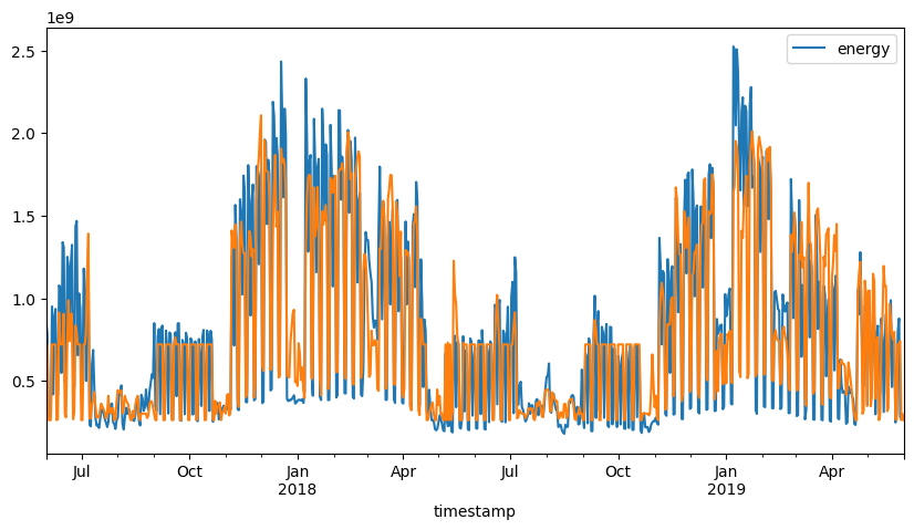
Adding the school holidays#
The previous categorisation of occupancy is not enough to explain the daily energy consumption. We need to add the school holidays to the model.
[16]:
%pip install vacances-scolaires-france jours-feries-france
Looking in indexes: https://pypi.org/simple, https://gitlab.ecoco2.com/api/v4/groups/recherche/-/packages/pypi/simple
Requirement already satisfied: vacances-scolaires-france in /home/ubuntu/mambaforge/envs/eat/lib/python3.11/site-packages (0.10.0)
Requirement already satisfied: jours-feries-france in /home/ubuntu/mambaforge/envs/eat/lib/python3.11/site-packages (0.7.0)
Note: you may need to restart the kernel to use updated packages.
[17]:
from jours_feries_france import JoursFeries
from vacances_scolaires_france import SchoolHolidayDates

jf = JoursFeries()
shd = SchoolHolidayDates()


def is_bank_holiday(date):
    return jf.is_bank_holiday(date)


def is_holiday(date):
    return shd.is_holiday_for_zone(date, "B")


def school_open_close(series: pd.Series):
    """Return a series of categories based on the day of the week of the index"""
    timestamps = series.index
    is_open = []
    for timestamp in timestamps:
        if timestamp.weekday() > 4:
            is_open.append("weekend")
        elif is_bank_holiday(timestamp.date()):
            is_open.append("weekend")
        elif is_holiday(timestamp.date()):
            is_open.append("holiday")
        else:
            is_open.append("Open")
    return pd.Series(data=is_open, index=series.index)
[18]:
data = pd.read_parquet(files[0]).loc[
    "2016-02-01":"2018-10-01"
]  # Selecting dates where the behaviour is more stable
categories = school_open_close(data)
display(categories.head())
display(categories.value_counts())
timestamp
2016-02-01 00:00:00+01:00    Open
2016-02-01 00:10:00+01:00    Open
2016-02-01 00:20:00+01:00    Open
2016-02-01 00:30:00+01:00    Open
2016-02-01 00:40:00+01:00    Open
dtype: object
Open       66240
weekend    43338
holiday    30672
Name: count, dtype: int64
[19]:
ts_holidays = CategoricalThermoSensitivity(
    energy_data=data["energy"],
    temperature_data=data["temperature"],
    categories=categories,
    frequency="1D",
    degree_days_type="auto",
    degree_days_computation_method="mean",
)
ts_holidays.fit()
display(ts_holidays.model.summary())
| Dep. Variable: | energy | R-squared: | 0.819 |
|---|---|---|---|
| Model: | OLS | Adj. R-squared: | 0.818 |
| Method: | Least Squares | F-statistic: | 877.3 |
| Date: | Fri, 11 Oct 2024 | Prob (F-statistic): | 0.00 |
| Time: | 20:44:41 | Log-Likelihood: | -19653. |
| No. Observations: | 974 | AIC: | 3.932e+04 |
| Df Residuals: | 968 | BIC: | 3.935e+04 |
| Df Model: | 5 | ||
| Covariance Type: | nonrobust |
| coef | std err | t | P>|t| | [0.025 | 0.975] | |
|---|---|---|---|---|---|---|
| heating_degree_days:Open | 8.125e+07 | 1.96e+06 | 41.464 | 0.000 | 7.74e+07 | 8.51e+07 |
| heating_degree_days:holiday | 8.248e+06 | 2.87e+06 | 2.874 | 0.004 | 2.62e+06 | 1.39e+07 |
| heating_degree_days:weekend | 4.009e+06 | 2.52e+06 | 1.589 | 0.112 | -9.42e+05 | 8.96e+06 |
| Intercept:Open | 2.965e+08 | 8.88e+06 | 33.375 | 0.000 | 2.79e+08 | 3.14e+08 |
| Intercept:holiday | 6.924e+07 | 1.12e+07 | 6.181 | 0.000 | 4.73e+07 | 9.12e+07 |
| Intercept:weekend | 6.59e+07 | 1.03e+07 | 6.403 | 0.000 | 4.57e+07 | 8.61e+07 |
| Omnibus: | 123.564 | Durbin-Watson: | 2.009 |
|---|---|---|---|
| Prob(Omnibus): | 0.000 | Jarque-Bera (JB): | 621.575 |
| Skew: | -0.462 | Prob(JB): | 1.06e-135 |
| Kurtosis: | 6.803 | Cond. No. | 7.90 |
Notes:
[1] Standard Errors assume that the covariance matrix of the errors is correctly specified.
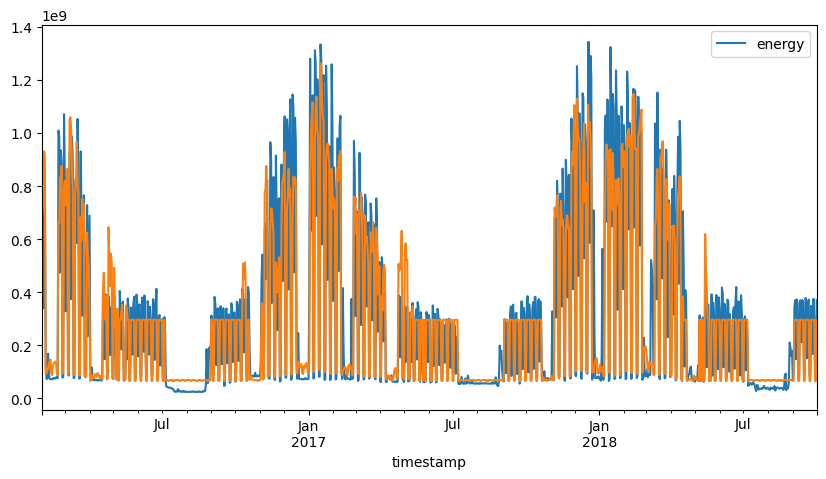
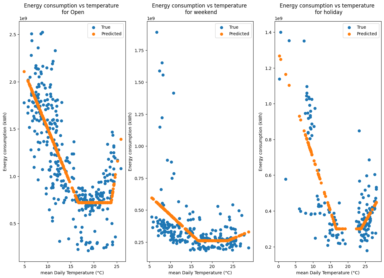
[20]:
fig, ax1 = plt.subplots(1, 1, figsize=(10, 5))
aggregated_data = ts_holidays.aggregated_data.dropna(how="any", axis=0)
aggregated_data[["energy"]].plot(ax=ax1)
predictions = ts_holidays.model.predict()
ax1.plot(aggregated_data.index, predictions, label="Predicted")
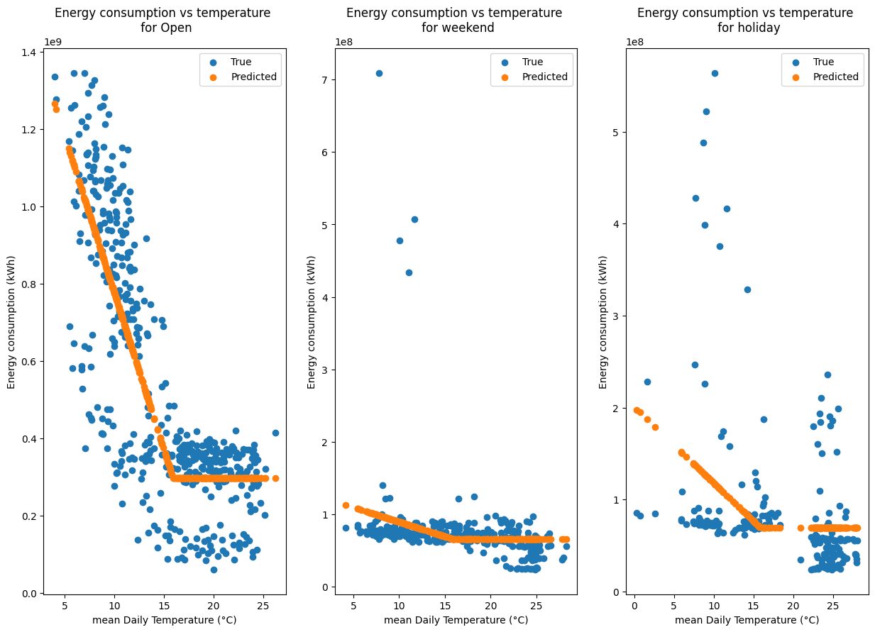
n_cat = len(categories.unique())
fig, axarr = plt.subplots(1, n_cat, figsize=(5 * n_cat, 10))
axarr = axarr.flatten() if n_cat > 1 else [axarr]
for i, cat in enumerate(categories.unique()):
mask = aggregated_data["category"] == cat
ax = axarr[i]
ax.scatter(
aggregated_data[mask]["temperature"],
aggregated_data[mask]["energy"],
label="True",
)
ax.scatter(
aggregated_data[mask]["temperature"], predictions[mask], label="Predicted"
)
ax.set_title(f"Energy consumption vs temperature \n for {cat}")
ax.set_xlabel("mean Daily Temperature (°C)")
ax.set_ylabel("Energy consumption (kWh)")
ax.legend()
[21]:
categories2 = school_open_close(data2)
display(categories2.head())
timestamp
2017-06-01 00:00:00+02:00    Open
2017-06-01 00:10:00+02:00    Open
2017-06-01 00:20:00+02:00    Open
2017-06-01 00:30:00+02:00    Open
2017-06-01 00:40:00+02:00    Open
dtype: object
[22]:
ts_holidays2 = CategoricalThermoSensitivity(
    energy_data=data2["energy"],
    temperature_data=data2["temperature"],
    categories=categories2,
    frequency="1D",
    degree_days_type="auto",
    degree_days_computation_method="mean",
)
ts_holidays2.fit()
display(ts_holidays2.model.summary())

fig, ax1 = plt.subplots(1, 1, figsize=(10, 5))
aggregated_data = ts_holidays2.aggregated_data.dropna(how="any", axis=0)
aggregated_data[["energy"]].plot(ax=ax1)
predictions = ts_holidays2.model.predict()

ax1.plot(aggregated_data.index, predictions, label="Predicted")

n_cat = len(categories2.unique())
fig, axarr = plt.subplots(1, n_cat, figsize=(5 * n_cat, 10))
axarr = axarr.flatten() if n_cat > 1 else [axarr]
for i, cat in enumerate(categories2.unique()):
    mask = aggregated_data["category"] == cat
    ax = axarr[i]
    ax.scatter(
        aggregated_data[mask]["temperature"],
        aggregated_data[mask]["energy"],
        label="True",
    )
    ax.scatter(
        aggregated_data[mask]["temperature"], predictions[mask], label="Predicted"
    )
    ax.set_title(f"Energy consumption vs temperature \n for {cat}")
    ax.set_xlabel("mean Daily Temperature (°C)")
    ax.set_ylabel("Energy consumption (kWh)")
    ax.legend()
| Dep. Variable: | energy | R-squared: | 0.787 |
|---|---|---|---|
| Model: | OLS | Adj. R-squared: | 0.784 |
| Method: | Least Squares | F-statistic: | 332.5 |
| Date: | Fri, 11 Oct 2024 | Prob (F-statistic): | 3.11e-236 |
| Time: | 20:44:58 | Log-Likelihood: | -15199. |
| No. Observations: | 731 | AIC: | 3.042e+04 |
| Df Residuals: | 722 | BIC: | 3.046e+04 |
| Df Model: | 8 | ||
| Covariance Type: | nonrobust |
| coef | std err | t | P>|t| | [0.025 | 0.975] | |
|---|---|---|---|---|---|---|
| heating_degree_days:Open | 1.177e+08 | 3.85e+06 | 30.561 | 0.000 | 1.1e+08 | 1.25e+08 |
| heating_degree_days:holiday | 5.941e+07 | 6.18e+06 | 9.606 | 0.000 | 4.73e+07 | 7.16e+07 |
| heating_degree_days:weekend | 3.016e+07 | 5.08e+06 | 5.942 | 0.000 | 2.02e+07 | 4.01e+07 |
| cooling_degree_days:Open | 3.163e+08 | 8.13e+07 | 3.893 | 0.000 | 1.57e+08 | 4.76e+08 |
| cooling_degree_days:holiday | 3.339e+07 | 1.85e+07 | 1.800 | 0.072 | -3.02e+06 | 6.98e+07 |
| cooling_degree_days:weekend | 1.371e+07 | 2.5e+07 | 0.548 | 0.584 | -3.54e+07 | 6.28e+07 |
| Intercept:Open | 7.199e+08 | 2.05e+07 | 35.128 | 0.000 | 6.8e+08 | 7.6e+08 |
| Intercept:holiday | 3.007e+08 | 3.35e+07 | 8.974 | 0.000 | 2.35e+08 | 3.67e+08 |
| Intercept:weekend | 2.615e+08 | 2.5e+07 | 10.463 | 0.000 | 2.12e+08 | 3.11e+08 |
| Omnibus: | 96.161 | Durbin-Watson: | 1.242 |
|---|---|---|---|
| Prob(Omnibus): | 0.000 | Jarque-Bera (JB): | 390.747 |
| Skew: | 0.542 | Prob(JB): | 1.41e-85 |
| Kurtosis: | 6.414 | Cond. No. | 31.0 |
Notes:
[1] Standard Errors assume that the covariance matrix of the errors is correctly specified.
Conclusion of Daily Analysis#
Using no category, the model is not able to capture the occupancy of the building. Using the day of week or the weekend is better, as more data is available for these categories, but their are some large discrepancies between the model and the data.
This may be due to the fact that the building is a school building and the school holidays are not taken into account.
Automatic Day categorisation#
The following section shows how to use the automatic days categorisation.
[23]:
from pandas import DataFrame
from energy_analysis_toolbox.thermosensitivity.daily_analysis import (
    AutoCategoricalThermoSensitivity,
)


ts_auto = AutoCategoricalThermoSensitivity(
    energy_data=data["energy"],
    temperature_data=data["temperature"],
    degree_days_type="auto",
    degree_days_computation_method="integral",
)
ts_auto.fit()
ts_auto
[23]:
AutoCategoricalThermoSensitivity(frequency=1D,
        degree_days_type=heating,
        degree_days_base_temperature={'heating': np.float64(17.18)},
        degree_days_computation_method=integral,
        interseason_mean_temperature=20)

                            OLS Regression Results
==============================================================================
Dep. Variable:                 energy   R-squared:                       0.606
Model:                            OLS   Adj. R-squared:                  0.601
No. Observations:                 974   F-statistic:                     113.5
Covariance Type:            nonrobust   Prob (F-statistic):          1.02e-183
=================================================================================================
                                    coef    std err          t      P>|t|      [0.025      0.975]
-------------------------------------------------------------------------------------------------
heating_degree_days:Friday     6.519e+07   4.79e+06     13.601      0.000    5.58e+07    7.46e+07
heating_degree_days:Monday     7.269e+07   4.72e+06     15.399      0.000    6.34e+07     8.2e+07
heating_degree_days:Saturday   1.876e+06   4.76e+06      0.394      0.693   -7.46e+06    1.12e+07
heating_degree_days:Sunday     1.747e+06   4.83e+06      0.362      0.718   -7.73e+06    1.12e+07
heating_degree_days:Thursday   6.525e+07   4.64e+06     14.063      0.000    5.61e+07    7.44e+07
heating_degree_days:Tuesday    6.511e+07   4.65e+06     13.991      0.000     5.6e+07    7.42e+07
heating_degree_days:Wednesday  3.289e+07   4.53e+06      7.265      0.000     2.4e+07    4.18e+07
Intercept:Friday               2.018e+08    2.4e+07      8.393      0.000    1.55e+08    2.49e+08
Intercept:Monday               2.043e+08   2.41e+07      8.493      0.000    1.57e+08    2.52e+08
Intercept:Saturday             6.484e+07   2.39e+07      2.716      0.007     1.8e+07    1.12e+08
Intercept:Sunday               6.367e+07    2.4e+07      2.650      0.008    1.65e+07    1.11e+08
Intercept:Thursday             2.014e+08   2.41e+07      8.361      0.000    1.54e+08    2.49e+08
Intercept:Tuesday                2.1e+08    2.4e+07      8.755      0.000    1.63e+08    2.57e+08
Intercept:Wednesday             8.94e+07    2.4e+07      3.719      0.000    4.22e+07    1.37e+08
=================================================================================================

Notes:
[1] Standard Errors assume that the covariance matrix of the errors is correctly specified.
[24]:
ts_auto.merge_and_fit()
ts_auto
[24]:
AutoCategoricalThermoSensitivity(frequency=1D,
        degree_days_type=heating,
        degree_days_base_temperature={'heating': np.float64(17.18)},
        degree_days_computation_method=integral,
        interseason_mean_temperature=20)

                            OLS Regression Results
==============================================================================
Dep. Variable:                 energy   R-squared:                       0.604
Model:                            OLS   Adj. R-squared:                  0.602
No. Observations:                 974   F-statistic:                     295.8
Covariance Type:            nonrobust   Prob (F-statistic):          4.58e-192
======================================================================================================================
                                                         coef    std err          t      P>|t|      [0.025      0.975]
----------------------------------------------------------------------------------------------------------------------
heating_degree_days:Monday-Tuesday-Thursday-Friday  6.705e+07   2.34e+06     28.593      0.000    6.24e+07    7.16e+07
heating_degree_days:Saturday-Sunday                 1.813e+06   3.38e+06      0.536      0.592   -4.83e+06    8.45e+06
heating_degree_days:Wednesday                       3.289e+07   4.52e+06      7.281      0.000     2.4e+07    4.18e+07
Intercept:Monday-Tuesday-Thursday-Friday            2.045e+08    1.2e+07     17.047      0.000    1.81e+08    2.28e+08
Intercept:Saturday-Sunday                           6.425e+07   1.69e+07      3.802      0.000    3.11e+07    9.74e+07
Intercept:Wednesday                                  8.94e+07    2.4e+07      3.727      0.000    4.23e+07    1.36e+08
======================================================================================================================

Notes:
[1] Standard Errors assume that the covariance matrix of the errors is correctly specified.
[25]:
fig, ax1 = plt.subplots(1, 1, figsize=(10, 5))
aggregated_data = ts_auto.aggregated_data.dropna(how="any", axis=0)
aggregated_data[["energy"]].plot(ax=ax1)
predictions = ts_auto.model.predict()

ax1.plot(aggregated_data.index, predictions, label="Predicted")

n_cat = len(ts_auto.resampled_categories.unique())
fig, axarr = plt.subplots(1, n_cat, figsize=(5 * n_cat, 10), sharey=True)
axarr = axarr.flatten() if n_cat > 1 else [axarr]
for i, cat in enumerate(ts_auto.resampled_categories.unique()):
    mask = aggregated_data["category"] == cat
    ax = axarr[i]
    ax.scatter(
        aggregated_data[mask]["temperature"],
        aggregated_data[mask]["energy"],
        label="True",
    )
    ax.scatter(
        aggregated_data[mask]["temperature"], predictions[mask], label="Predicted"
    )
    ax.set_title(f"Energy consumption vs temperature \n for {cat}")
    ax.set_xlabel("mean Daily Temperature (°C)")
    if i == 0:
        ax.set_ylabel("Energy consumption (kWh)")
    ax.legend()
[26]:
ts_auto2 = AutoCategoricalThermoSensitivity(
    energy_data=data2["energy"],
    temperature_data=data2["temperature"],
    degree_days_type="auto",
    degree_days_computation_method="integral",
)
ts_auto2.fit()
ts_auto2.merge_and_fit()
ts_auto2
[26]:
AutoCategoricalThermoSensitivity(frequency=1D,
        degree_days_type=heating,
        degree_days_base_temperature={'heating': np.float64(17.97)},
        degree_days_computation_method=integral,
        interseason_mean_temperature=20)

                            OLS Regression Results
==============================================================================
Dep. Variable:                 energy   R-squared:                       0.629
Model:                            OLS   Adj. R-squared:                  0.627
No. Observations:                 731   F-statistic:                     246.3
Covariance Type:            nonrobust   Prob (F-statistic):          1.33e-153
======================================================================================================================
                                                         coef    std err          t      P>|t|      [0.025      0.975]
----------------------------------------------------------------------------------------------------------------------
heating_degree_days:Monday-Tuesday-Thursday-Friday  9.722e+07   4.06e+06     23.941      0.000    8.92e+07    1.05e+08
heating_degree_days:Saturday-Sunday                 2.474e+07   5.91e+06      4.186      0.000    1.31e+07    3.63e+07
heating_degree_days:Wednesday                        8.77e+07   7.91e+06     11.090      0.000    7.22e+07    1.03e+08
Intercept:Monday-Tuesday-Thursday-Friday            6.002e+08   2.39e+07     25.115      0.000    5.53e+08    6.47e+08
Intercept:Saturday-Sunday                           2.554e+08   3.35e+07      7.627      0.000     1.9e+08    3.21e+08
Intercept:Wednesday                                  2.76e+08   4.85e+07      5.686      0.000    1.81e+08    3.71e+08
======================================================================================================================

Notes:
[1] Standard Errors assume that the covariance matrix of the errors is correctly specified.
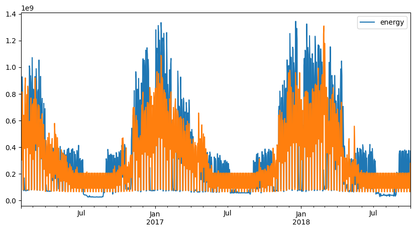
[27]:
fig, ax1 = plt.subplots(1, 1, figsize=(10, 5))
aggregated_data = ts_auto2.aggregated_data.dropna(how="any", axis=0)
aggregated_data[["energy"]].plot(ax=ax1)
predictions = ts_auto2.model.predict()
ax1.plot(aggregated_data.index, predictions, label="Predicted")
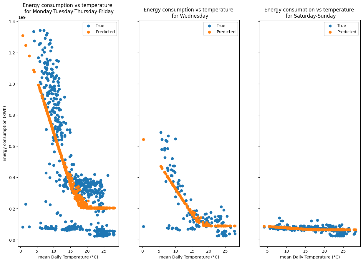
n_cat = len(ts_auto2.resampled_categories.unique())
fig, axarr = plt.subplots(1, n_cat, figsize=(5 * n_cat, 10), sharey=True)
axarr = axarr.flatten() if n_cat > 1 else [axarr]
for i, cat in enumerate(ts_auto2.resampled_categories.unique()):
mask = aggregated_data["category"] == cat
ax = axarr[i]
ax.scatter(
aggregated_data[mask]["temperature"],
aggregated_data[mask]["energy"],
label="True",
)
ax.scatter(
aggregated_data[mask]["temperature"], predictions[mask], label="Predicted"
)
ax.set_title(f"Energy consumption vs temperature \n for {cat}")
ax.set_xlabel("mean Daily Temperature (°C)")
if i == 0:
ax.set_ylabel("Energy consumption (kWh)")
ax.legend()
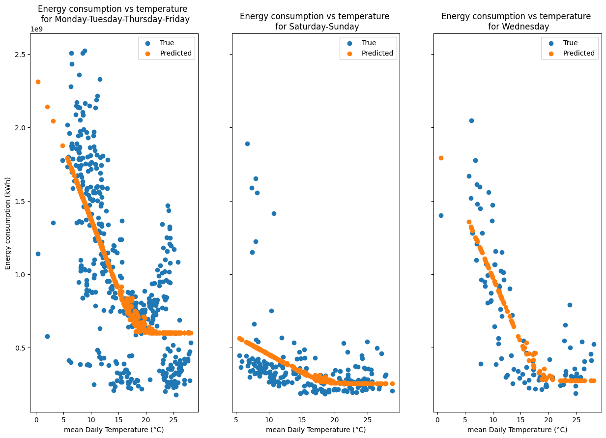
Conclusion of Automatic Day categorisation#
As you can see, the model is able to detect that the building has three different occupancy categories: - usual school days Monday, Tuesday, Thursday, Friday - usual weekends Saturday, Sunday - Wednesdays
However, the effect of the holidays is not taken into account in this implementation.
Conclusion#
As you can see, in contrast with synthetic data, the different days behaviors due to different building occupancy leads to multiple thermosensitivity model.
Discussion / Next steps#
The next step would be to improve the classifications. For instance, we can re-label the periods according to the observed energy consumption. One way to do so is the following: - compute the predicted energy consumption of the period for each category - estimate the probability of each category given the energy consumption of the period and the standard deviation of the energy consumption of the category - re-label the periods with the category with the highest probability (Max a posteriori estimation)
However, this cannot be used to detect unexpected occupancy, on the contrary.
Another way would be an unsupervised classification of the periods. But for now this is a be too complex for the model.